This is the fourth part of a series. See parts 1, 2, 3, and 5. Comments are open on this post.

What good are markets anyway? Why should we rely upon them to make economic decisions about what gets produced and who gets what, rather than, say, voting or having an expert committee study the matter and decide? Is there a value-neutral, “scientific” (really “scientifico-liberal“) case for using markets rather than other mechanisms? Informally, we can have lots of arguments. One can argue that most successful economies rely upon market allocation, albeit to greater and lesser degrees and with a lot of institutional diversity. But that has not always been the case, and those institutional differences often swamp the commonalities in success stories. How alike are the experiences of Sweden, the United States, Japan, current upstarts like China? Is the dominant correlate of “welfare” really the extensiveness of market allocation, or is it the character of other institutions that matters, with markets playing only a supporting role? Maybe the successes are accidental, and attributing good outcomes to this or that institution is letting oneself be “fooled by randomness“. History might or might not make a strong case for market economies, but nothing that could qualify as “settled science”.

But there is an important theoretical case for the usefulness of markets, “scientific” in the sense that the only subjective value it enshrines is the liberal presumption that what a person would prefer is ipso facto welfare-improving. This scientific case for markets is summarized by the so-called “welfare theorems“. As the name suggests, the welfare theorems are formalized mathematical results based on stripped-down and unrealistic models of market economies. The ways that real economies fail to adhere to the assumptions of the theorems are referred to as “market failures”. For example, in the real world, consumers don’t always have full information; markets are incomplete and imperfectly competitive; and economic choice is entangled with “externalities” (indirect effects on people other than the choosers). It is conventional and common to frame political disagreements around putative market failures, and there’s nothing wrong with that. But for our purposes, let’s set market failures aside and consider the ideal case. Let’s suppose that the preconditions of the welfare theorems do hold. Exactly what would that imply for the role of markets in economic decisionmaking?

We’ll want to consider two distinct problems of economic decisionmaking, Pareto-efficiency and distribution. Are there actions that can be taken which would make everyone better off, or at least make some people better off and nobody worse off? If so, our outcome is not Pareto efficient. Some unambiguous improvement from the status quo remains unexploited. But when one person’s gain (in the sense of experiencing a circumstance she would prefer over the status quo) can only be achieved by accepting another person’s loss, who should win out? That is the problem of distribution. The economic calculation problem must concern itself with both of those dimensions.

We have already seen that there can be no value-neutral answer to the distribution problem under the assumptions of positive economics + liberalism. If we must weigh two mutually exclusive outcomes, one of which would be preferred by one person, while the other would be preferred by a second person, we have no means of making interpersonal comparisons and deciding what would be best. We will have to invoke some new assumption or authority to choose between alternatives. One choice is to avoid all choices, and impose as axiom that all Pareto efficient distributions are equally desirable. If this is how we resolve the problem, then there is no need for markets at all. Dictatorship, where one person directs all of an economy’s resources for her own benefit, is very simple to arrange, and, under the assumptions of the welfare theorems, will usually lead to a Pareto optimal outcome. (In the odd cases where it might not, a “generalized dictatorship” in which there is a strict hierarchy of decision makers would achieve optimality.) The economic calculation problem could be solved by holding a lottery and letting the winner allocate the productive resources of the economy and enjoy all of its fruits. Most of us would judge dictatorship unacceptable, whether imposed directly or arrived at indirectly as a market outcome under maximal inequality. Sure, we have no “scientific” basis to prefer any Pareto-efficient outcome over any other, including dictatorship. But we also have no basis to claim all Pareto-efficient distributions are equivalent.

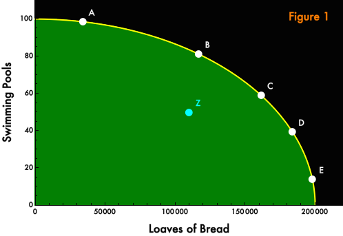
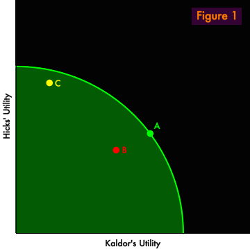
Importantly, we have no basis even to claim that all Pareto-efficient outcomes are superior to all Pareto-inefficient distributions. For example, in Figure 1, Point A is Pareto-efficient and rankably superior to Pareto-inefficient Point B. Both Kaldor and Hicks prefer A over B. But we cannot say whether Point A is superior or inferior to Point C, even though Point A is Pareto-efficient and Point C is not. Kaldor prefers Point A but Hicks prefers Point C, its Pareto-inefficiency notwithstanding. The two outcomes cannot be ranked.

We are simply at an impasse. There is nothing in the welfare theorems, no tool in welfare economics generally, by which to weigh distributional questions. In the next (and final) installment of our series, we will try to think more deeply about how “economic science” might be put to helpfully address the question without arrogating to itself the role of Solomon. But for now, we will accept the approach that we have already seen Nicholas Kaldor and John Hicks endorse: Assume a can opener. We will assume that there exist political institutions that adjudicate distributional tradeoffs. In parliaments and sausage factories, the socially appropriate distribution will be determined. The role of the economist is to be an engineer, Keynes’ humble dentist, to instruct on how to achieve the selected distribution in the most efficient, welfare-maximizing way possible. In this task, we shall see that the welfare theorems can be helpful.

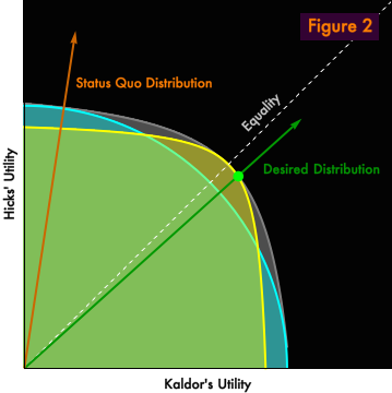
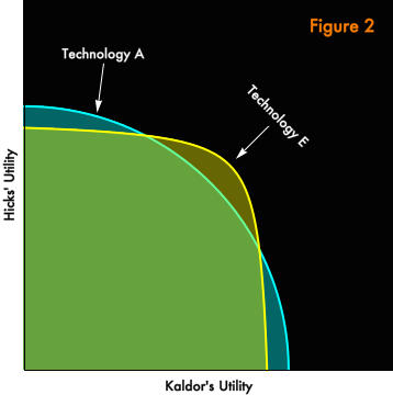
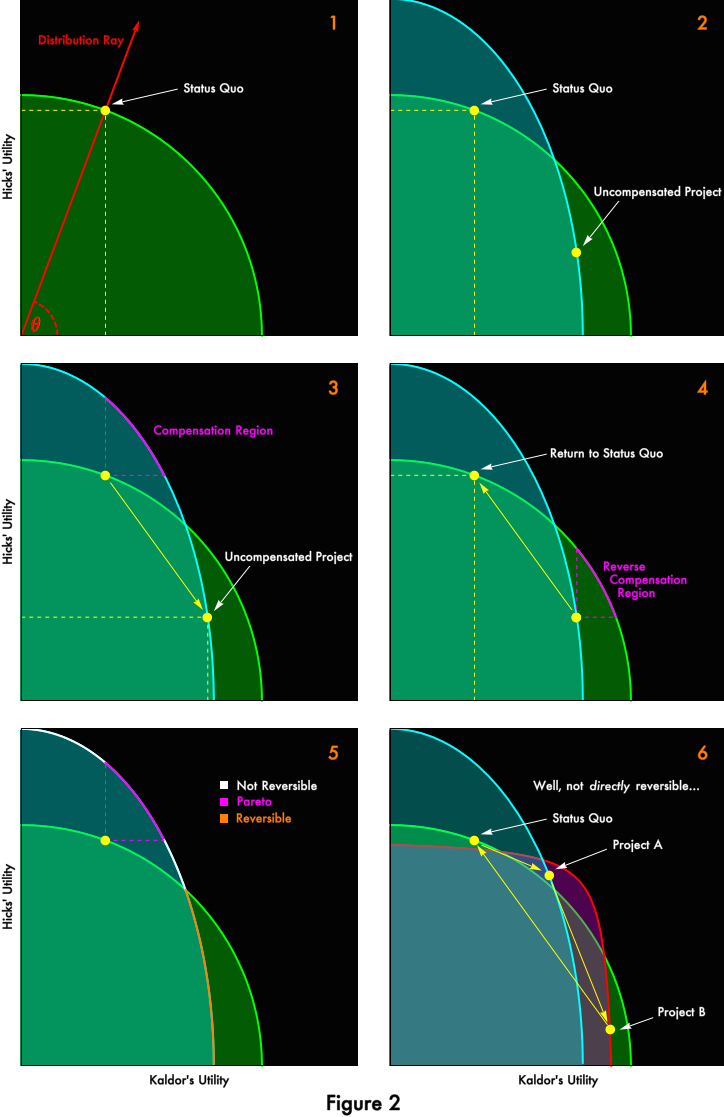
Figure 2 is a re-presentation of the two-person economy we explored in the previous post. Kaldor and Hicks have identical preferences, under a production function where different distributions will lead to deployment of different technologies. In the previous post, we explored two technologies, discrete points on the production possibilities frontier, and we will continue to do so here. However, we’ve added a light gray halo to represent the continuous envelope of all possible technologies. (The welfare theorems presume that such a continuum exists. The halo represents the full production possibilities frontier from the Figure 1 of the previous post. The yellow and light blue curves represent specific points along the production frontier.) Only two technologies will concern us because only two distributions will concern us. There is the status quo distribution, which represented by the orange ray. But the socially desired distribution is represented by the green ray. Our task, as dentist-economists, is to bring the economy to the green point, the unique Pareto-optimal outcome consistent with the socially desired distribution.

If economic calculation were easy, we could just make it so. Acting as benevolent central planners, we would select the appropriate technology, produce the set of goods implied by our technology choice, and distribute those goods to Kaldor and Hicks in Pareto-efficient quantities consistent with our desired distribution. But we will concede to Messrs. von Mises and Hayek that economic calculation is hard, that as central planners, however benevolent, we would be incapable of choosing the correct technology and allocating the goods correctly. Those choices depend upon the preferences of Kaldor and Hicks, which are invisible and unknown to us. Even if we could elicit consumer preferences somehow, our calculation would become very complex in an economy containing many more than two people and a near infinity of goods. We’d probably screw it up.

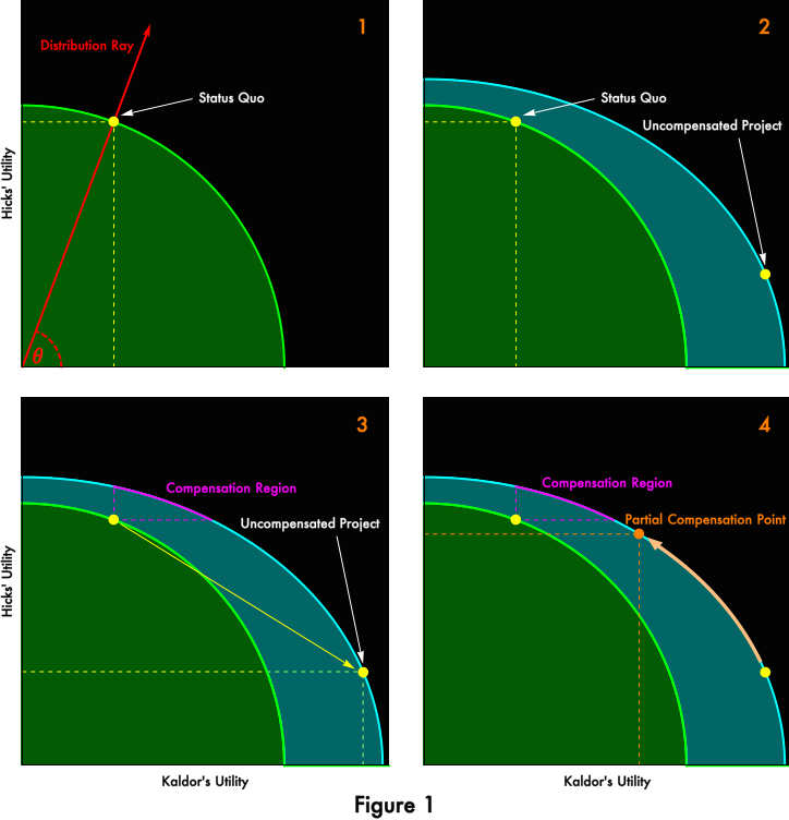
Enter the welfare theorems. The first welfare theorem tells us that, in the absence of “market failure” conditions, free trade under a price system will find a Pareto-efficient equilibrium for us. The second welfare theorem tells us that for every point in the “Pareto frontier”, there exists a money distribution such that free trade under a price system will take us to this point. We have been secretly using the welfare theorems all along, ever since we defined distributions as rays, fully characterized by an angle. Under the welfare theorems, we can characterize distributions in terms of money rather than worrying about quantities of specific goods, and we can be certain that each point on a Pareto frontier will map to a distribution, which motivates the geographic representation as rays. The second welfare theorem tells us how to solve our economic calculation problem. We can achieve our green goal point in two steps. (Figure 3) First, we transfer money from Hicks to Kaldor, in order to achieve the desired distribution. Then, we let Kaldor and Hicks, buy, sell, and trade as they will. Price signals will cause competitive firms to adopt the optimal technology (represented by the yellow curve), and the economy will end up at the desired green point.

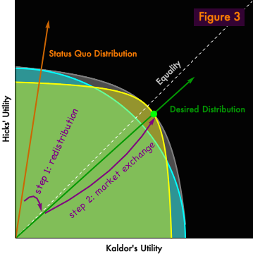
The welfare theorems are often taken as the justification for claims that distributional questions and market efficiency can be treated as “separate” concerns. After all, we can choose any distribution, and the market will do the right thing. Yes, but the welfare theorems also imply we must establish the desired distribution prior to permitting exchange, or else markets will do precisely the wrong thing, irreversibly and irredeemably. Choosing a distribution is prerequisite to good outcomes. Distribution and market efficiency are about as “separable” as mailing a letter is from writing an address. Sure, you can drop a letter in the mail without writing an address, or you can write an address on a letter you keep in a drawer, but in neither case will the letter find its recipient. The address must be written on the letter before the envelope is mailed. The fact that any address you like may be written on the letter wouldn’t normally provoke us to describe these two activities as “separable”.

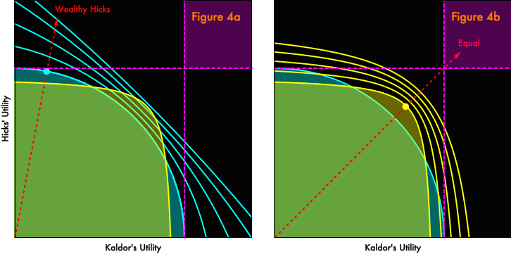
Figure 4 illustrates the folly of the reverse procedure, permitting market exchange and then setting a distribution.

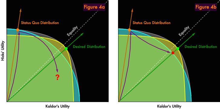
In both panels, we first let markets “do their magic”, which take us to the orange point, the Pareto-efficient point associated with the status quo distribution. Then we try to redistribute to the desired distribution. In Panel 4a, we face a very basic problem. The whole reason we required markets in the first place was because we are incapable of determining Pareto-efficient distributions by central planning. So, if we assume that we have not magically solved the economic calculation problem, when we try to redistribute in goods ex post (rather than in money ex ante), we are exceedingly unlikely to arrive at a desirable or Pareto efficient distribution. In Panel 4b, we set aside the economic calculation problem, and presume that we can, somehow, compute the Pareto-efficient distribution of goods associated with a distribution. But we’ll find that despite our remarkable abilities, the best that we can do is redistribute to the red point, which is Pareto-inferior to the should-be-attainable green point. Why? Because, in the process of market exchange, we selected the technology optimal for the status quo distribution (the light blue curve) rather than the technology optimal for the desired distribution (the yellow curve). Remember, our choice of “technology” is really the choice of which goods get produced and in what quantities. Ex post, we can only redistribute the goods we’ve actually produced, not the goods we wish we would have produced. There is no way to get to the desired green point unless we set the distribution prior to market exchange, so that firms, guided by market incentives, select the correct technology.

The welfare theorems, often taken as some kind of unconditional paean to markets, tell us that market allocation cannot produce a desirable Pareto-efficient outcome unless we have ensured a desirable distribution of money and initial endowments prior to market exchange. Unless you claim that Pareto-efficient allocations are lexicographically superior to all other allocations, that is, unless you rank any Pareto-efficient allocation as superior to all not Pareto-efficient distributions — an ordering which reflects the preferences of no agent in the economy — unconditional market allocation is inefficient. That is to say, unconditional market allocation is no more or less efficient than holding a lottery and choosing a dictator.

In practice, of course, there is no such thing as “before market allocation”. Markets operate continuously, and are probably better characterized by temporary equilibrium models than by a single, eternal allocation. The lesson of the welfare theorems, then, is that at all times we must restrict the distribution of purchasing power to the desired distribution or (more practically) to within an acceptable set of distributions. Continuous market allocation while the pretransfer distribution stochastically evolves implies a regime of continuous transfers in order to ensure acceptable outcomes. Otherwise, even in the absence of any conventional “market failures”, markets will malfunction. They will provoke the production of a mix of goods and services that is tailored to a distribution our magic can opener considers unacceptable, goods and services that can not in practice or in theory be redistributed efficiently because they poorly suited to more desirable distributions.

By the way, if you think that markets themselves should choose the distribution of wealth and income, you are way off the welfare theorem reservation. The welfare theorems are distribution preserving, or more accurately, they are distribution defining — they give economic meaning to money distributions by defining a deterministic mapping from those distributions to goods and services produced and consumed. Distributions are inputs to a process that yields allocations as outputs. If you think that the “free market” should be left alone to determine the distribution of wealth and income, you may or may not be wrong. But you can’t pretend the welfare theorems offer any help to your case.

There is nothing controversial, I think, in any of what I’ve written. It is all orthodox economics. And yet, I suspect it comes off as very different from what many readers have learned (or taught). The standard introductory account of “market efficiency” is a parade of plain fallacies. It begins, where I began, with market supply and demand curves and “surplus”, then shows that market equilibria maximize surplus. But “surplus”, defined as willingness to pay or willingness to sell, is not commensurable between individuals. Maximizing market surplus is like comparing 2 miles against 12-feet-plus-32-millimeters, and claiming the latter is longest because 44 is bigger than 2. It is “smart” precisely in the Shel Siverstein sense. More sophisticated catechists then revert to a compensation principle, and claim that market surplus is coherent because it represents transfers that could have been made, the people whose willingness to pay is measured in miles could have paid off the people whose willingness to pay is measured in inches, leaving everybody better off. But, as we’ve seen, hypothetical compensation — the principle of “potential Pareto improvements” — does not define an ordering of outcomes. Even actual compensation fails to redeem the concept of surplus: the losers in an auction, paid-off much more than they were willing to pay for an item as compensation for their loss, might be willing to return the full compensation plus their original bid to gain the item, if their original bid was bound by a hard budget constraint, or (more technically) did not reflect an interior solution to their constrained maximization problem. No use of surplus, consumer or producer, is coherent or meaningful if derived from market (rather than individual) supply or demand curves, unless strong assumptions are made about transactors’ preferences and endowments. The welfare theorems tell us that market allocations will not produce outcomes that are optimal for all distributions. If the distribution of wealth is undesirable, markets will misdirect capital and make poor decisions with respect to real resources even while they maximize perfectly meaningless “surplus”.

So, is there a case for market allocation at all, for price systems and letting markets clear? Absolutely! The welfare theorems tell us that, if we get the distribution of wealth and income right, markets can solve the profoundly difficult problem of converting that distribution into unfathomable multitudes of production and consumption decisions. The real world is more complex than the maths of welfare theorems, and “market failures” can muddy the waters, but that is still a great result. The good news in the welfare theorems is that markets are powerful tools if — but only if — the distribution is reasonable. There is no case whatsoever for market allocation in the absence of a good distribution. Alternative procedures might yield superior results to a bad Pareto optimum under lots of plausible notions of superior.

There are less formal cases for markets, and I don’t necessarily mean to dispute those. Markets are capable of performing the always contentious task of resource allocation with much less conflict than alternative schemes. Market allocation with tolerance of some measure of inequality seems to encourage technological development, rather than the mere technological choice foreseen by the welfare theorems. In some institutional contexts, market allocation may be less corruptible than other procedures. There are lots of reasons to like markets, but the virtue of markets cannot be disentangled from the virtue of the distributions to which they give effect. Bad distributions undermine the case for markets, or for letting markets clear, since price controls can be usefully redistributive.

How to think about “good” or “bad” distributions will be the topic of our final installment. But while we still have our diagrams up, let’s consider a quite different question, market legitimacy. Under what distributions will market allocation be widely supported and accepted, even if we’re not quite sure how to evaluate whether a distribution is “right”? Let’s conduct the following thought experiment. Suppose we have two allocation schemes, market and random. Market allocation will dutifully find the Pareto-efficient outcome consistent with our distribution. Random allocation will place us at an arbitrary point inside our feasible set of outcomes, with uniform probability of landing on any point. Under what distributions would agents in our economy prefer market to random allocation?

Let’s look at two extremes.

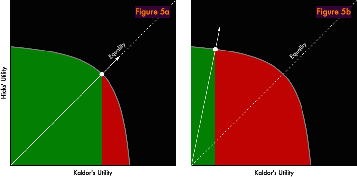
In Panel 5a, we begin with a perfectly equal distribution. The red area delineates a region of feasible outcomes that would be superior to the market allocation from Kaldor’s perspective. The green area marks the region inferior to market allocation. The green area is much larger than the red area. Under equality, Kaldor strongly prefers market allocation to alternatives that tend to randomize outcomes. “Taking a flyer” is much more likely to hurt Kaldor than to help him.

In Panel 5b, Hicks is rich and Kaldor is poor under the market allocation. Now things are very different. The red region is much larger than the green. Throwing some uncertainty into the allocation process is much more likely to help Kaldor than to hurt. Kaldor will rationally prefer schemes that randomize outcomes in favor of determinstic market allocation. He will prefer such schemes knowing full well that it is unlikely that a random allocation will be Pareto efficient. You can’t eat Pareto efficiency, and the only Pareto-efficient allocation on offer is one that’s worse for him than rolling the dice. If Kaldor is a rational economic actor, he will do his best to undermine and circumvent the market allocation process. Note that we are not (necessarily) talking about a revolution here. Kaldor may simply support policies like price ceilings, which tend to randomize who gets what amid oversubscribed offerings. He may support rent control and free parking, and oppose congestion pricing. He may prefer “fair” rationing of goods by government, even of goods that are rival, excludable, informationally transparent, and provoke no externalities. Kaldor’s behavior need not be taken as a comment on the virtue or absence of virtue of the distribution. It is what it is, a prediction of positive economics, rational maximizing.

Of course, if Kaldor alone is unhappy with market allocation, his hopes to randomize outcomes are unlikely to have much effect (unless he resorts to outright crime, which can be rendered costly by other channels). But in a democratic polity, market allocation might become unsupportable if, say, the median voter found himself in Kaldor’s position. Now we come to conjectures that we can try to quantify. How much inequality-not-entirely-in-his-interest would Kaldor tolerate before turning against markets? What level of wealth must the median voter have to prevent a democratic polity from working to circumvent and undermine market allocation?

Perfect equality is, of course, unnecessary. Figure 6, for example, shows an allocation in which Kaldor remains much poorer than Hicks, yet Kaldor continues to prefer the market allocation to a random outcome.

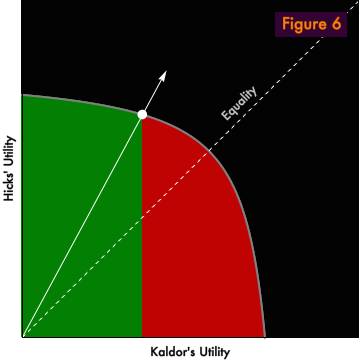
We could easily compute from our diagram the threshold distribution below which Kaldor prefers random to market allocation, but that would be pointless since we don’t live in a two-person ecomomy with a utility possibilities curve I just made up. With a little bit of math [very informal: pdf nb], we can show that for an economy of risk-neutral individuals with identical preferences under constant returns to scale, as the number of agents goes to infinity the threshold value beneath which random allocation is preferred to the market tends to about 69% of mean income. (Risk neutrality implies constant marginal utility, enabling us map to from utility to income.) That is, people in our simplified economy support markets as long as they can claim at least 69% of what they would enjoy under an equal distribution. This figure is biased upwards by the assumption of risk-neutrality, but it is biased downwards by the assumption of constant returns to scale. Obviously don’t take the number too seriously. There’s no reason to think that the magnitude of the biases are comparable and offsetting, and in the real world people have diverse preferences. Still, it’s something to think about.

According the the Current Population Survey, at the end of 2012, median US household income was 71.6% of mean income. But the Current Population Survey fails to include data about top incomes, and so its mean is an underestimate. The median US household likely earns well below 69% of the mean.

If it is in fact the case that the median voter is coming to rationally prefer random claims over market allocation, one way to support the political legitimacy of markets would be to compress the distribution, to reduce inequality. Another approach would be to diminish the weight in decision-making of lower-income voters, so that the median voter is no longer the “median influencer” whose preferences are reflected by the political system.

Note: There will be one more post in this series, but I won’t get to it for at least a week, and I’ve silenced commenters for way too long. Comments are (finally!) enabled. Thank you for your patience and forbearance.

This is the third part of a series. See parts 1, 2, 4, and 5.

Last time, we concluded that output cannot be measured independently of distribution, “the size of the proverbial pie in fact depends upon how you slice it.” That’s a clear enough idea, but the example that we used to get there may have seemed forced. We invented people with divergent circumstances and preferences, and had a policy decision rather than “the free market” slice up the pie.

Now we’ll consider a more natural case, although still unnaturally oversimplified. Imagine an economy in which only two goods are produced, loaves of bread and swimming pools. Figure 1 below shows a “production possibilities frontier” for our economy.

The yellow line represents locations of efficient production. Points A, B, C, D, and E, which sit upon that line, are “attainable”, and the production of no good can be increased without a corresponding decrease in the other good. Point Z is also attainable, but it is not efficient: by moving from Z to B or C, more of both goods could be made available. Assuming (as we generally have) that people prefer more goods to fewer (or that they have the option of “free disposal”), points B and C are plainly superior to point Z. However, from this diagram alone, there is no way to rank points A, B, C, D, and E. Is possibility A, which produces a lot of swimming pools but not so much bread, better or worse than possibility E, which bakes aplenty but builds pools just a few?

Under the usual (dangerous) assumptions of “base case” economics — perfect information, complete and competitive markets, no externalities — markets with profit-seeking firms will take us to somewhere on the production possibilities frontier. But precisely which point will depend upon the preferences of the people in our economy. How much bread do they require or desire? How much do they like to swim? How much do they value not having to share the pools that they swim in? Except in very special cases, which point will also depend upon the distribution of wealth among the people in our economy. Suppose that the poor value an additional loaf of bread much more than they value the option of privately swimming, while the rich have full bellies, and so allocate new wealth mostly towards personal swimming pools. Then if wealth is very concentrated, the market allocation will be dominated by the preferences of the wealthy, and we’ll end up at points A or B. If the distribution is more equal and few people are so sated they couldn’t do with more bread, we’ll find points D or E. All of the points represent potential market allocations — we needn’t posit any state or social planner to make the choice. But the choice will depend upon the wealth distribution.

Let’s try to understand this in terms of the diagrams we developed in the previous piece. We’ll contrast points A and E as representing different technologies. Don’t mistake this for different levels of technology. We are not talking about new scientific discoveries. By a “technology” we simply mean an arrangement of productive resources in the world. One technology might involve devoting a large share of productive resources to the construction of very efficient large-scale bakeries, while another might redirect those resources to the mining and mixing of the materials in concrete. Humans, whether via markets or other decision-making institutions, can choose either of these technologies without anyone having to invent things. (By happenstance, Paul Krugman drew precisely this distinction yesterday.)

Figure 2 shows a diagram of Technology A and Technology E in our two person (“Kaldor” and “Hicks”) economy.

The two technologies are not rankable independently of distribution. I hope that this is intuitive from the diagram, but if it is not, read the previous post and then persuade yourself that the two orange points in Figure 3 below are subject to “Scitovsky reversals”. One can move from either orange point to the other, and it would be possible to compensate the “loser” for the change in a way that would leave both parties better off. So, by the potential Pareto criterion, each point is superior to the other, there is no well-defined ordering.

In contrast to our previous example of an unrankable change, Kaldor and Hicks here have identical and very natural preferences. Both devote most of their income to bread when they are poor but shift their allocation towards swimming pool construction as they grow rich. As a result, both prefer Technology A when the distribution of wealth is lopsided (the light blue points), while both prefer Technology E (the yellow point) when the distribution is very equal. It’s intuitive, I think, that whoever is rich prefers swimming-pool-centric Technology A. What may be surprising is that, if the wealth distribution is held constant, the choice of technology is always unanimous. If Hicks is rich and Kaldor is poor, even Kaldor prefers Technology A, because his meager share of the pie includes claims on swimming pools that he can offer to The Man in exchange for disproportionate quantities of bread.

This is more obvious if we consider an extreme. Suppose there were a technology that produced all bread and no swimming pools under a very unequal wealth distribution. Then, putting aside complications like altruism, whoever is rich eats a surfeit of bread that provides almost no satisfaction, and perhaps even throws away a large excess. The poor have nothing but bread to trade for bread, so there is no trade. They are stuck with no way to expand the small meals they are endowed with. But, add some swimming pools to the economy and give the poor a pro rata share of everything (i.e. define the initial distribution in terms of money), then all of a sudden the poor have something that the rich value, which they can exchange for excess bread that the rich value not at all. The rich are willing to surrender a lot of (useless to them) bread in exchange for even small claims on the swimming pools that they really want. When things are very unequal, the benefit to the poor of having something to trade exceeds the cost of an economy whose aggregate production is not well matched with their consumption. Aggregate production goes to the rich; the poor are in the business of maximizing their crumbs.

So, which organizations of resources, Technology A or Technology E, is “most efficient”, “maximizes the size of the pie”? There is no distribution-independent answer to that question. If the pie will be sliced up equally, then Technology E is superior. If the pie will be sliced up very unequally, then Technology A is superior. The size of the pie depends upon how you slice it, given very natural, very ordinary sorts of preferences. Patterns of resource utilization, of what gets produced and what does not, depend very much on the distribution of wealth within an economy. It’s not coherent to claim that economic arrangements are “more efficient” than they would be under some alternative distribution. If what you mean by “efficiency” is mere Pareto efficiency, there are Pareto-efficient outcomes consistent with any distribution. If you have a broader notion of economic efficiency in mind, then which arrangements are “most efficient” cannot be defined independently of the distribution of wealth.

I’ll end with a speculative thought experiment, about technological development. Remember, up until now, we’ve been considering alternative choices among already known technologies. Now let’s think about the relationship between distribution and the invention of new technologies. Consider Figure 4 below:

In our two-person economy, technological improvement shifts utility possibility curves outward, making it feasible for both individuals to increase their enjoyment without any tradeoff. In Figure 4, we have shown outward shifts from the two technologies that we considered above. Panel 4a shows incremental improvements on Technology A. Panel 4b shows incremental improvements on Technology E. Not all technological improvements are incremental, but most are, even most of what gets marketed as “revolutionary”. We assume, per the discussion above, that our economy chooses the distribution-dependent superior technology and iterates from that. We also assume that, absent political intervention, the deployment of new technology leaves the distribution of wealth pretty much unchanged. That may or may not be realistic, but it will serve as a useful base case for our thought experiment.

In both panels, after four iterative improvements, technological improvement dominates the choice of technologies in a rankable Kaldor-Hicks sense. After four rounds of technological change, regardless of which technology we started from, there is some distribution under the new technology that would be a Pareto improvement over any feasible distribution prior to the technological development. (My choice of four iterations is completely arbitrary; this is just an illustration.) If we assume that adoption of the new technology is accompanied by optimal social choice of distribution (however the “optimality” of that choice is defined), technological improvement quickly overwhelms the initial, distribution-dependent, choice of technology. A futurist, technoutopian view naturally follows: whatever sucks about now, technological change will undo it, overcome it.

But “optimal social choice of distribution” is a hard assumption to swallow. What if we suppose, more realistically, inertia — that there’s a great deal of status quo bias in distributive institutions, that the distribution after technology adoption remains similar to the distribution prior. Worse, but realistically, what if we imagine that distribution-preserving technological change and redistribution are perceived within political institutions as alternative means of addressing economically induced unhappiness and dissatisfaction, as substitutes rather than complements. Some voices hail “innovation” as the solution to problems like poverty and precarity, while other voices argue that redistribution, however contentious, represents a surer path.

Under what circumstances would distribution-preserving innovation dominate distributional conflict as a strategy for overcoming economic discontent? A straightforward criterion would be when technological change could yield outcomes better than any change in distributional arrangements or choice of status quo technologies. In Figure 4 (both panels), this dominant region is represented by the purple region northeast of the purple dashed lines.

Distribution-preserving innovation implies moving outward with technological change along the current “distribution ray”, represented by the red dashed line. Qualitatively, loosely, informally, the distance that one would have to travel along a distribution ray before intersecting with the dominant region is a measure of the plausibility of innovation as a universally acceptable alternative to distributional conflict. The shorter the distance from the status quo to the dominant technology region, the more attractive innovation, rather than distributional conflict, becomes for all parties. Conversely, if the distance from the status quo to a sure improvement is very long, one party is likely to find contesting distributive arrangements a more plausible strategy than supporting innovation.

In the right-hand panel of Figure 4, representing an equal current distribution, innovation along the distribution ray would pretty quickly reach the dominant region. Just a few more rounds than are shown and the yellow-dot status quo could travel along the red-dashed distribution ray to the purple promised land. But in the left-hand panel, where we start with a very unequal distribution, the distribution ray would not intersect the purple region for a long, long time, well beyond the top boundary of the figure. When the status quo is this unequal, innovation is unlikely to be a credible alternative to distributional conflict. In the limiting case of a perfectly unequal distribution, the distribution ray would sit at 90° (or 0°) and even infinite innovation would fail to intersect the redistribution-dominating region. For the status quo loser, no possible distribution-preserving innovation would be superior to contesting distributional arrangements.

For agents with similar preferences, more equal distributions will be “closer” to the dominant region for three reasons:

• perfect equality is “minimax“, that is it minimizes the maximum benefit achievable by either party from redistribution, reducing the attractiveness of distributive fights;
• under equality, for a given level of technology, the choice among available technologies will fall closer (or at least as close) to the dominant region as under less equal distributions, giving iterations from that choice a head start;
• the closest-in point of the dominant region (the point closest to the origin) sits on the equal-distribution ray, it is there that one finds the “lowest hanging fruit”. More unequal “distribution rays” point to ever more distant frontiers of the dominant region.

Note that there is a continuum, not a stark choice between perfectly equal and very unequal distributions. The more equal the distribution of wealth, the more attractive will be innovation as an alternative to distributive conflict. As the distribution of wealth becomes more unequal, distributive losers will come to perceive calls for innovation as a fig-leaf that distracts from a more contentious but superior strategy, while distributive winners will preach technoutopianism with ever greater fervor.

There’s lots to argue with in our little thought experiment. Technological change needn’t be distribution-preserving, innovation and redistribution needn’t be mutually exclusive priorities, the “distance” in our diagrams — in joint utility space along contours of technological change — may defy the Euclidean intuitions I’ve invited you to indulge. Nevertheless, I think there’s a consonance between our story and the current politics of technology and innovation. The best way to build a consensus in favor of innovation and technological development may be to address distributional issues that make cynics of potential enthusiasts.

Note: With continued apologies, comments remain closed until the completion of this series of posts on welfare economics. Please do write down your thoughts and save them! I think there will be two more posts, with comments finally open on the last.

This is the second part of a series. See parts 1, 3, 4, and 5.

When economics tried to put itself on a scientific basis by recasting utility in strictly ordinal terms, it threatened to perfect itself to uselessness. Summations of utility or surplus were rendered incoherent. The discipline’s new pretension to science did not lead to reconsideration of its (unscientific) conflation of voluntary choice with welfare improvement. So it remained possible for economists to recommend policies that would allow some people to be made better off (in the sense that they would choose their new circumstance over the old), so long as no one was made worse off (no one would actively prefer the status quo ante). “Pareto improvements” remained defensible as welfare-improving. But, very little of what economists had previously understood to be good policy could be justified under so strict a criterion. Even the crown jewel of classical liberal economics, the Ricardian case for free trade, cannot meet the test. As John Hicks memorably put it, the caution implied by the new “economic positivism might easily become an excuse for the shirking of live issues, very conducive to the euthanasia of our science.”

Hicks, following Nicholas Kaldor and Harold Hotelling, thought he had a way out. Suppose there were an economy that, in isolation, could produce 50 bottles of wine and 40 bolts of cloth. If the borders were opened, the country would specialize in wine-making. Devoting its full capacity to the task, it would produce enough wine so as to be able to keep 60 bottles for domestic use, even while trading for a full 50 bolts of cloth. Under the presumption that people prefer more to less, “the economy” would clearly be made better off by opening the borders. There would be more wine and more cloth “to go ’round”. However, in practice, skilled cloth-makers would be impoverished by the change. They would be reemployed as menial grape-pickers, leading to a reduction of earnings so great that they’d have less cloth and less wine to consume, despite the increase in overall wealth. Opening the borders is not a Pareto improvement: the “pie” grows larger, but some people are made badly worse off. So, on what basis might a “scientific” economist recommend the policy?

The insight that Kaldor, Hicks, and Hotelling brought to the problem is simple. Opening the borders represents a potential Pareto improvement, if we imagine that those who benefit from the change compensate those who lose out. In our example, since the total quantities of wine and cloth available are greater with free trade than without, there must be some way of distributing the bounty that leaves everyone at least as well off as they were before, and others better off. Economists could, in good conscience, argue for policies that would be Pareto improvements, if they were bundled with some redistribution, regardless of whether or not the redistribution would, in the event, actually happen. Such a change is now said to be “Kaldor-Hicks efficient“, or, more straightforwardly, a “Potential Pareto improvement”.

At first blush, this sounds dumb. Nobody harmed by a change can eat a “potential” Pareto improvement. But there is, nonetheless, a case to be made for the criterion. The distribution of scarce goods and services is inherently a question of competing values. But quantities of goods are objective and measurable. So a “scientific” economics could concern itself with “efficiency” — maximizing objective economic output, while the distribution of that output and concerns about “equity” could be left to the political institutions that adjudicate competing values. An activity that could leave everybody with all the goods and services they might otherwise have while providing some people with even more necessarily implies an increase in the quantity of goods and services made available, and is objectively superior on efficiency grounds. If those goods and services get distributed poorly, that may be a terrible problem. But it represents a failure of politics, and outside the scope of a scientific economics. Let economics concern itself with the objective problem of maximizing output, and remain silent on the inherently political question of how output should be distributed.

This is might be a clever answer to the threat of the “euthanasia of our science”, but it is incoherent as the basis for a welfare economics. In reality, economic output cannot be objectively measured. The quantity of corn or cars or manicures produced can be counted. An action that increases the availability of all goods, actual and potential, might be pronounced an objective increase in the size of the economy. But most economic activities provoke tradeoffs in production: more of something gets produced, while less of something else does. There is no way to determine whether such an event represents an increase or decrease in the size of the economy without making interpersonal comparisons of value. Dollar values can’t be used in place of goods and services unless the dollars actually change hands, prices change to reflect the new patterns of wealth and production, and all parties consent that their new situation is superior to the old. When there are trade-offs made in patterns of production, only an actual Pareto improvement counts as an objective increase in the size of an economy.

Tibor de Scitovsky demonstrated very elegantly the incoherence of Kaldor-Hicks efficiency in a world with multiple goods. I’m going to present the argument in detail, stealing a pedagogical trick from Matthew Adler and Eric Posner, but adding my own overdone diagrams.

Let’s start charitably. Figure 1 shows some pictures of the special case that might be scored as an objective increase in efficiency:

We have an economy of two people, Nicholas Kaldor and John Hicks. In Panel 1, the bright green curve represents a “utility possibilities curve“. For each point on the curve, the x value represents “how much utility” Kaldor enjoys while the y value represents how much Hicks enjoys. Utility is strictly ordinal, so the axes are unlabeled, and the exact shapes are meaningless. You could stretch or squeeze the diagram as much as you like, rescale it to any aspect ratio, and nothing would change. Any transformation that preserves the x– and -ordering of things is fine.

At a given time, the economy is represented by a point on the curve. Each location reflects a different distribution of economic output. The point where the curve intersects the y-axis represents an economy in which Hicks gets literally all of the goods, while Kaldor dies starving. As we rotate clockwise along the curve, Hicks gets less and less, while Kaldor gets more and more. Again, the exact shape is meaningless. All we can tell is that, as control over economic output shifts, Hicks’ utility declines while Kaldor’s rises. Finally we reach the x-axis, where it is Kaldor who starves while Hicks feasts. At the moment, the economy sits at the yellow point marked “status quo”.

A distribution can be summarized by the angle marked θ in Panel 1. When θ is 0°, Kaldor owns the whole economy. When θ is 90°, Hicks owns everything. We can locate Kaldor’s and Hicks’ satisfaction under any distribution by following the “distribution ray” to the utility possibilities curves. [1]

In Panel 2, a policy change is proposed. It might be deployment of a new technology, or construction of high return infrastructure. But let’s imagine that it trade-liberalization under circumstances where Ricardian comparative advantage logic unproblematically holds.

It turns out that John Hicks is a skilled cloth-maker. That’s how he earns an honest living. If trade were liberalized, textile manufacture would be outsourced, and he would be out of a job. Nicholas Kaldor, on the other hand, owns acres and acres of vineyards. His real income would dramatically increase, as cloth would grow cheaper and the market for his wine would expand. If the borders were simply thrown open, the economy would end up at the position marked “Uncompensated Project” in Panel 2. Trade liberalization is not Pareto improving. As you can see, relative to the status quo, we shift rightwards (Kaldor benefits big time!) but also downwards (Hicks loses) if the project is implemented without compensating redistribution. Can we state, as a matter of objective science rather than value judgment, that trade-liberalization would represent an efficiency improvement?

Kaldor, Hicks, and Hotelling ask us to perform a thought experiment represented on Panel 3. Suppose that we did throw open the borders. We’d be thrust along the yellow arrow from the current status quo to the new “uncompensated project” point. Would it be possible to redistribute along the new utility possibilities frontier in a way that would render the policy-change-plus-redistribution a Pareto improvement, a boon both for Kaldor and for Hicks? The existence of the purple region, above and to the right of our original status quo, shows that it is indeed possible. Our trade liberalization is a “potential Pareto improvement”, and should be scored by economists an objective efficiency gain, regardless of whether not the political institutions that adjudicate rival claims actually impose compensation. Political institutions might not compensate Hicks at all, leaving him where he lands in Panel 3. Or they might compensate only partially, as in Panel 4. Maybe it is best to retain market incentives for fogies like Hicks to anticipate change and learn new skills. Maybe the resentment that would be provoked by full compensation overwhelms the benefit of making Hicks whole. Maybe there is no good reason, but the political system is plagued by inertia and so fails to compensate. Or maybe Kaldor has bought the politicians with his good wine. Those are questions beyond the scope of economic science. Nevertheless, say Kaldor, Hotelling, even penurous Hicks, we can objectively declare the proposed policy an efficiency improvement. If poor Hicks starves when all is said and done, well, that will be the fault of the politicians. Or perhaps it will be optimal. As economists, we really can’t say. Incomparable subjectivities are involved.

I have to admit to feeling queasy about this, like a surgeon who opens the chest of an awake screaming patient and then blames the anesthesiologist for sleeping in. But this is the procedure Kaldor and Hicks propose for us. (Hotelling, to his great credit, admits the possibility that imperfect politics might imply revision of his economic prescriptions.) But we’ll put our reservations aside for now, and declare this policy change an “efficiency increase”, distinct and separable from distributional concerns.

Now let’s examine a different project. Hicks has abandoned his cloth-making (a folly of youth!) and has entered a respectable profession, bourbon distillery. Kaldor, never a fool, has stuck with his wine-making.

Here is the thing, though. Each gentleman has come to despise the good he himself produces. The grapes stain Kaldor’s fingers, his clothes, his bare soles. Hicks is plagued by the smell of corn mash and the weight of oak barrels. If Hicks were a rich man, he’d never look at a bottle of bourbon. He’d sip wine like a gentleman. If Kaldor were a rich man, he would drown the nightmares (out, out, damned wine stain!) in a bottle of whiskey.

In Panel 1 of Figure 2, we start very much like before. Kaldor and Hicks ply their trades, they get what they get, represented in joint utility terms by the yellow-dot status quo.

In Panel 2, a rezoning of some land is considered, which would prevent “industrial agriculture” on acreage currently devoted to the growing of corn. There’d be nothing for this land but to transition it to bucolic vineyards. Both of our protagonists are ambivalent about the proposal. In his role as producer, the rezoning would be great for Kaldor’s business. Hicks would have to sell the land for a song, enabling more and cheaper wine production. But the rezoning would shift the composition of output in a manner opposed to Kaldor’s consumption preferences. If Kaldor could be made rich in some manner independent of the proposed change — if we drew a “distribution ray” in Panel 2 at 0° signifying Kaldor’s complete ownership of output — Kaldor would strongly prefer the status quo and the abundant bourbon it produces to the proposed repurposing of land for wine. Conversely, the businessman in Hicks hates the proposal, selling out to Kaldor for a song would really sting! But the wine-lover in Hicks would be delighted, if only he’d be rich enough to afford the wine. If the “distribution ray” were at 90° — if Hicks was very rich — he’d strongly prefer that the land be rezoned!

So, can economic science tell us whether the rezoning is efficient? According to Messrs. Kaldor, Hicks, and Hotelling (when they dabble at economics), the proposal is efficient. In Panel 3, you can see that, subsequent to the rezoning, it would be possible to redistribute output in a manner that would leave both parties better off than the status quo, exactly as in Panel 3 of Figure 1 above! The change would survive any cost-benefit analysis.

But. Here comes Mr. Scitovsky, who is a real sourpuss. He points out (Panel 4) that, subsequent to the rezoning, analysis under the very same criterion would declare a reversal of the rezoning efficient! Does it make sense to declare the rezoning an “increase in economic efficiency” and then to declare the undoing another increase in economic efficiency? I have an idea: Get the zoning authority to to re-re-re-re-re-re-rezone the land. We’ll have so many economic efficiency increases, all scarcity will be vanquished!

Or not. What Scitovsky showed, quite definitively, is that the Potential Pareto criterion is incoherent as a measure of economic efficiency. It just doesn’t work. In a fallen world, it may in practice be used to evaluate potential changes, just as in a fallen world interpersonal comparisons of utility are used to evaluate changes. Both are equally (un)scientific under the axioms of liberal economics. Scitovsky proved that, in general, it is simply not possible to score the efficiency of a change without taking into account effects both on output and on distribution. The two are not independent, except in the special case illustrated by Figure 1.

Scitovsky didn’t think he was destroying the Potential Pareto criterion entirely. He pointed out that, for some distributions, reversals are not possible. Panel 5 of Figure 2 divides the utility possibilities frontier after the proposed change into distributions that are Pareto-improving (which implies making actual, full compensation for the change), into regions that are reversable and therefore not rankable as efficiency improvements, and into regions that are Potential Pareto but not Pareto and still irreversible. Scitovsky thought that changes that led to these distributions might still scored as efficiency increasing under Kaldor-Hicks-Hotelling logic. It took subsequent work to show that, no, even these irreversible regions aren’t safe. (See Blackorby and Donaldson for a mathematical review.) Scitovsky’s proposed modification of the Kaldor-Hicks criterion is intransitive, permitting cycles if more than two projects are compared. Project A can be “more efficient” than the status quo, Project B can be “more efficient” than Project A, but the status quo can be “more efficient” that Project B. Hmm. Panel 6 of Figure 2 shows an example. I won’t go through it in detail, but if you’ve understood the diagrams, you should be able to persuade yourself that 1) each transition is both Kaldor-Hicks efficient and irreversible; 2) there is no coherent efficiency ordering between them.

While it is impossible to rank alternatives at arbitrary distributions, it is possible to rank projects if we fix a distribution. In Figure 2, Panel 2, extend a “distribution ray” outward from the origin at any angle. The outermost project is preferred. At a slight angle, when Kaldor enjoys most of the output, the bourbon-producing status quo is preferable. At a steep angle, when it is Hicks who will do most of the consuming, the wine-drenched rezoning is preferable. There is some distribution where both Kaldor and Hicks would be indifferent to the proposed rezoning, where the curves cross.

Given the rather elaborate story we told to rationalize the shape of the curves in Figure 2, you might wonder whether we might rescue a “scientific” efficiency from value-laden distributional concerns by suggesting that these “reversals” and “intransitivities” are rare, pathological cases that can in practice be ignored. They are not. We will encounter a simpler example soon. The likelihood that these sorts of issues arise increases with the number of people and goods in an economy, unless you restrict the form of peoples’ utility functions unrealistically. Allowing for (nearly) unrestricted preferences (people are assumed always to prefer more goods to less or to have the option of “free disposal”), the only projects that can be ranked independently of distribution are those that increase the number of some goods and services without any cost in availability of other goods or services, an analog to Pareto efficiency in the sphere of production.

As one economist put it:

The only concrete form that has been proposed for [a social welfare function grounded in ordinal utilities] is the compensation principal developed by Hotelling. Suppose the current situation is to be compared with another possible situation. Each individual is asked how much he is willing to pay to change to the new situation; negative amounts mean that the individual demands compensation for the change. The possible situation is said to be better than the current one if the algebraic sum of all the amounts offered is positive. Unfortunately, as pointed out by T. de Scitovsky, it may well happen that situation B may be preferred to situation A when A is the current situation, while A may be preferred to B when B is the current situation.

Thus, the compensation principal does not provide a true ordering of social decisions. It is the purpose of this note to show that this phenomenon is very general.

That economist was Kenneth Arrow. “This note“, circulated at The Rand Corporation, was the first draft of what later become known as Arrow’s Impossibility Theorem.

It is not, actually, an obscure result, this impossibility of separating “efficiency” from distribution. The only place you will not find it is in most introductory economics textbooks, which describe an “equity” / “efficiency” trade-off without pointing out that the size of the proverbial pie in fact depends upon how you slice it.

I wonder why that is missing.

Note: This was the second of a series of posts on welfare economics. The first was here. With apologies, I’m disabling comments until the end of the series, so I can get through my little plan untempted by the brilliant and enticing diversions that I know commenters would offer. Please do write down your comments, and save them for the final post in the series. I thought this would go faster; I feel very guilty for leaving no forum for responses for so long. I really am sorry about that!