So this will be an unusual post, more picture book than essay. Plus, it’s interactive! If you are willing to install the Mathematica plug-in, you can be the central banker / fiscal authority of your very own graphical economy!

As readers may have noticed, I’ve been thinking lately about Keynesian and monetarist business cycle theories. I don’t mean to wholly endorse these theories. I’ve some sympathy for Austrian-ish or “recalculationist” ideas too. But I do think there’s merit in the idea that recessions frequently occur because aggregate expenditure is, for whatever reason, inadequate. I’ve been frustrated by all the squabbles, between self-styled Keynesians and post-Keynesians, academic defenders of mainstream central banking and the more risqué internet “quasimonetarists”. My view is that these groups are more alike than different in their economic ideas, but that they manufacture controversies to signal political affiliations and institutional preferences regarding how and by whom policy decisions should be made.

So, I’ve been trying to understand the ways in which these theories are alike and different, and organize my own thinking about how to evaluate different policy proposals. I’m a pretty visual thinker, but for a variety of reasons, I’ve never found the most common ways to diagram Keynesian ideas — IS/LM and AS/AD — especially helpful. In my mind, I found myself falling back on Econ 101 style supply and demand graphs, where the commodity of interest, whose “price” and quantity is to be determined, is nominal expenditure. I’m sure this is not a novel approach, but I’ve gotten a lot of mileage out of it. Perhaps you won’t find it entirely useless.

The hardest part is to make sense of the basic set-up, so let’s talk it through.

The Basics

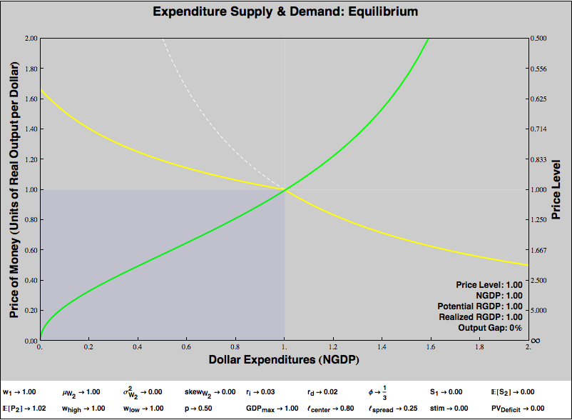
Below is a diagram of an economy in which demand shortfalls do not lead to output losses and money is neutral, because there are no price rigidities.

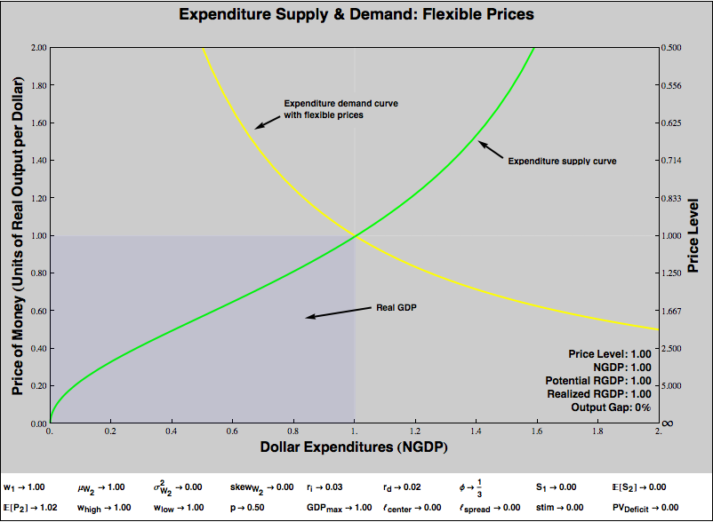
The downward-sloping yellow line is a demand curve, and the upward-sloping green line is a supply curve. Hopefully that seems familiar. However, we’re in a bit of a mirror universe, because we are graphing the supply and demand of expenditure. So the “expenditure suppliers”, represented by the green curve, are economic consumers. They supply dollars, for a “price”, which is some quantity of real goods and services. The “expenditure demanders” are economic producers. They demand dollars, but are only willing to offer so many goods and services for a buck. The equilibrium, the point where the two lines intersect, shows the price of a dollar, in real goods and services, that equalizes producers’ demand for money and consumers willingness to supply it.

For example, suppose that, at equilibrium, you can buy two widgets for a dollar. So the price of a widget is 50¢. But the price of a dollar is two widgets! Note the relationship — the dollar price of widgets is

(1 / PRICE_OF_DOLLARS_IN_WIDGETS)

This relationship is reflected on the axes if the graph. The left axis shows the price of money in real goods. If money is “expensive”, if you have to offer a lot of real stuff to get a dollar, that corresponds to a low price level, think deflation. Conversely, if money is “cheap” — if the equilibrium falls towards the bottom of the graph — then that means goods and services are expensive, think inflation. The right-hand axis shows the conventional price level, which rises as you travel vertically down the graph. As the price of money in real goods and services falls to 0, so you’d give up a dollar for next to nothing, the price level on the right-hand axis rises to infinity.

The X or quantity axis of the graph indicates how many dollars will be spent at the equilibrium. This has a very natural interpretation as nominal GDP. So, from the equilibrium point on the graph, we can read the price level (on the right axis) and the nominal GDP directly.

Real GDP is represented by the area of the bluish rectangle in the bottom left corner of the graph. To understand why, recall that real GDP is just

(NGDP / PRICE_LEVEL)

But the Y axis of the graph is

(1 / PRICE_LEVEL)

So the area of the bluish rectangle is

NGDP × (1 / PRICE_LEVEL) = (NGDP / PRICE_LEVEL) = RGDP

So what determines the shape of the expenditure supply and demand curves? Let’s start with demand. Suppose the economy produces at capacity and there are no “rigidities” to prevent the sale of all output. Producers will always accept however many dollars are on offer and sell the maximum achievable RGDP. Then

NGDP × (1 / PRICE_LEVEL) = MAX_RGDP
(1 / PRICE_LEVEL) = (MAX_RGDP / NGDP)

Since the inverse price level is our Y axis, and NGDP is our X axis, the function that describes our no-rigidity demand curve is just

Y = (MAX_RGDP / X)

which is the graph of a grade-school hyperbola. We’ll modify this shape a bit, when we start thinking about price rigidity. But let’s hold off on that.

What determines the shape of expenditure supply? That’s where all of the action is in terms of fiscal and monetary policy, and we’ll graph lots of funky shapes below. But fundamentally, the answer to this question is easy. Imagine a world of consumers, each of whom must decide how much to spend now and how much to save for the future. Suppose we can characterize consumers’ “intertemporal preferences” with a utility function. Then we can compute how much each consumer will spend. Naturally, that utility function will take into account the current price level, among other parameters. If we hold other parameters constant, we can compute how expenditure varies with the current level of prices. We add up all consumers’s expnditures and plot them on the X axis, against (1 / PRICE_LEVEL) on the Y axis. That gives us our expenditure supply curve.

Immaculate Deflation

In the graph above, everything has been normalized to one. The graph shows one unit of real goods “buying” one dollar of expenditures, for a price level of one. Suppose that consumers become more reluctant to spend money, that is, they perceive the marginal opportunity cost of parting with money as increasing. The result would be an “immaculate deflation”, in that expenditure would fall, but so would the price level, so that the reduced expenditure would still purchase all the economy’s real product, and RGDP would not fall at all. Here’s the graph:

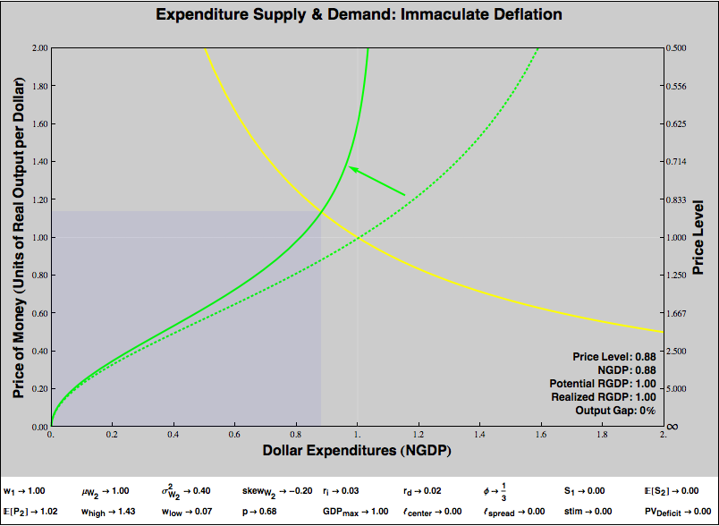
Note expenditures have fallen, but the quantity of goods offered for each dollar has risen. Real GDP — the area of the bluish rectangle — has not changed.

Price Rigidity

In the real world, when nominal expenditures fall, the quantity of goods offered for a dollar doesn’t rise enough to compensate. The quantity of goods purchased actually decreases. Let’s graph that:

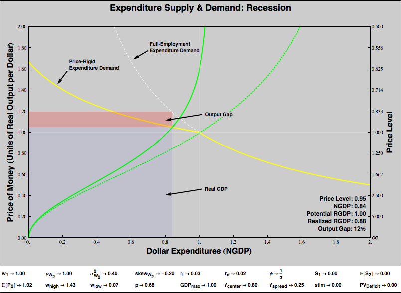
The expenditure supply curve is identical to that in the previous graph. However, the shape of the expenditure demand curve has changed. There is now a “kink”, that begins (as I’ve drawn it) just under the original equilibrium expenditure of one. Our steepened expenditure supply hits the kinked region, forcing that the quantity of goods offered for a dollar to be lower — or the price level to be higher — than in the previous graph, with its unkinked, flexible-price expenditure demand curve. This means that, given the reduced level of expenditure (caused, as before, by the steepening of the expenditure supply curve), the quantity of goods consumers purchase is less than the economy’s capacity. We observe a fall in real GDP and a recession.

As before, the area of the bluish rectangle represents Real GDP. The dotted white line shows the flexible-price expenditure demand curve, while the yellow line is the expenditure demand curve that actually obtains, with its kink and price rigidity. The reddish rectangle represents the output gap: the area that should have formed part of GDP, but does not because of the price rigidity.

In this example, the price level has from 1 to 0.96 (a 4% deflation), and real GDP has fallen by 10%. Note that in the previous example, with the same steepened expenditure supply curve but flexible prices, the price level fell even farther (to 0.88, a 12% deflation), but RGDP was unaffected. There’s an important bit of intuition here. We often imagine that deflation causes recessions, and indeed in our graph, we can see that deflation is associated with recessions. We would only see an output gap when the equilibrium fell before the kink in the curve, which is always a price level lower than our original price level. But under flexible pricing, the deflation would have been more severe, without harming RGDP. It is not too much deflation that creates the output gap, but too little deflation given the fall in expenditures! Tepid deflation is a marker of recessions, but it is the decline in nominal expenditure, in NGDP, that drives the show.

If you are wondering where the shape of the sticky-price expenditure demand curve comes from, see my earlier post on sticky prices. Basically, to generate the expenditure demand curve with price rigidity, I assume that industry leverage is uniformly distributed over some range, that firms in industries set minimum prices based in their degree of leverage, and that firms’ capacity is constrained in the short term. If you don’t buy that story, but agree that prices are sticky downward but not so sticky upward, then you can take the shape as an arbitrary qualitative depiction of that.

The Expenditure Supply Curve

Expenditure supply is where the action is in making sense of Keynesian and monetarist interventions. The nice thing about this framework is one can posit any intertemporal utility function you like for agents in your economy and then compute the shape of the expenditure supply curve as you vary parameters.

For the purpose of this exercise, I’ll adopt an unrealistic but illustrative utility function presumed to be shared by all consumers. Consumers will face a two period, rather than infinite horizon optimization problem. Their behavior will be based upon a number of factors, all of which are treated as exogenous parameters:

• An interest rate r_i which determines the Period 2 value of money not spent in Period 1.
• An current wage w₁, in nominal dollars.
• An expected future wage μ_w2, in nominal dollars.
• Variance of the distribution of future wages, σ_w2²
• Skewness of the distribution of future wages, skew_w2
• A current price level P₁
• An expected future price level E[P₂]. (Oddly, the current price level is what we are trying do determine. The expected future price level is known, and helps to pin the present price level.)
• A current taxes-and-transfers surplus S₁.
• An expected future taxes-and-transfers surplus E[S₂].
• A discount rate r_d, which is the rate at which consumers discount future utility.

A “real” model wouldn’t treat all these parameters as free. For example, perhaps the expected price level is dependent upon current interest rates, or fiscal policy. My goal here isn’t to present a falsifiable model of consumer behavior, but to illustrate what proponents of various interventions are claiming, and explore under what circumstances they would or wouldn’t work. We will find, for example, that, running a Period 1 taxes-and-transfers deficit while holding interest rates constant increases Period 1 expenditures. However, this effect will be mostly undone if the Period 1 deficit must be balanced by a Period 2 surplus. We don’t wish to take a position here in the “Ricardian equivalence” debate. Allowing the two deficit parameters to vary freely, rather than enforcing some hypothesized relationship, permits us to illustrate the claims of partisans on both sides.

The utility function I’m using to compute the expenditure supply function is shown below.

Our variable x represents nominal dollar expenditures.

There are a bunch of things about this utility function that are crappy, but I think it’s good enough to show how changes in parameters might affect a expenditure supply curve, and offer some intuition about how various interventions might work.

Although I’m using just one utility function here, a nice thing about this framework is that it need not rely on a representative agent. What we will derive, after all, is a Marshallian supply curve. We can define populations of agents with different parameters or preferences and combine the supply curves by “horizontal addition”.

Visualizing Changes in Expenditure Supply

Let’s start with a graph of an economy characterized by price rigidity, but which is currently at “full employment equilibrium”. (The scare quotes are because I am not explicitly modeling labor, so by full employment I just mean that the economy is producing at capacity.)

Now, suppose that for whatever reason, uncertainty surrounding future wages increases:

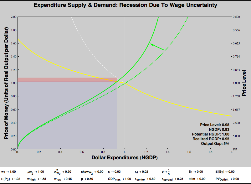
The expenditure supply curve steepens. Consumers become more reluctant to part with dollars, as they have been made worse off in the future and prefer to save. Unfortunately, after this steepening, the expenditure supply curve now intersects with the sticky-prices region of the expenditure demand curve. The resulting equilibrium is recessionary; the economy experiences a 5% output gap.

What kind of interventions might we try to fix this? Conventionally, our first resort is to discourage financial saving and promote current expenditures by reducing interest rates:

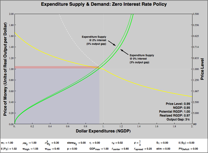
Dropping interest rates to zero helps, but it turns out to be insufficient, a 3% output gap remains. We have entered the liquidity trap, if you believe in such a thing.

But we are certainly not out of potential of interventions. Suppose we believe that the central bank is very, very good at setting expectations. Okay, if it were really great at that, it could just reverse the shock to consumers’ expectations of wage uncertainty and we’d never leave our initial equilibrium. But suppose the central bank can’t do that, but it can manage expectations of the price level. Then…

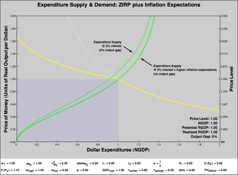
That worked! Yay monetary policy, still potent at the zero bound! But, we should be careful. We’ve assumed the central bank could set price level expectations. That’s much less sure than assuming it can set interest rates. Plus, perhaps engineering an uptick in inflation expectations is hazardous. Perhaps the central bank cannot set expectations precisely, so that there is a hazard of overshooting and generating inflation rather than just restoring equilibrium. Perhaps there is value to keeping inflation expectations “anchored”, and the change in expectations required to restore equilibrium would upset that anchoring. So, it’s worth considering alternatives.

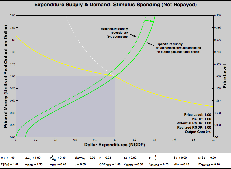
Let’s go back to our original disequilibrium, and let the MMT-ers have their way. Suppose that to counter the 5% output gap, the government reduced taxes and/or increased transfers, to run a deficit. Could that work? Absolutely.

However, there’s a catch. My two period setup is pretty Ricardian. Encouraging private spending through a taxes and transfers deficit in Period 1 only works if that deficit is not repaid by running a surplus in Period 2.

However, in the real world, deficits needn’t be repaid via prompt surpluses, and economies (measured in nominal dollars) often grow faster than the interest rate paid on public debt. In this case, debt effectively repays itself over time, without ever requiring surpluses. The core new debate over MMT as well as a very old debate over “Ricardian equivalence” turn on the degree to which people have (or by tax policy can be made to have) a special willingness to hold currency and government securities even when doing so implies an opportunity cost relative to a hypothetical asset that matches the economy’s growth rate. I think the case is very strong that, under many circumstances, people are willing to bear that cost, not least because a hypothetical asset that earns the economy’s growth rate with little risk does not exist, and most people are more concerned with managing risk than with maximizing return.

(Note: If you think transfers that will never be paid for in taxes must increase the expected future price level, then in the immediate term, all that does is to reduce the scale of the program necessary to eliminate the output gap! An increase future price level expectations, like the unfinanced transfer itself, renders the expenditure supply curve shallower, helping carry our equilibrium out of the recession region. Of course, we are observing a one period snapshot of the economy, and there may be long-term bad consequences to “unanchoring” the price level. That’s beyond the scope of our little visualization, but that doesn’t mean we shouldn’t worry about it.)

My little experiment is not so friendly to a taxes-and-transfers-based “hard Keynesianism“, which prescribes prompt surpluses to offset cyclical deficits. In my toy model, a reduction of expected future income is very much like a reduction of present income, as agents can borrow and save at “the” interest rate. But this is not realistic: real humans pay more to save than to borrow, and may face outright credit rationing.

I give lip service to uncertainty by calling the future surplus “expected”, but I don’t actually model it as uncertain, as wages are the only random variable in my toy utility function. If I had, the cost of future surpluses to consumers would be even greater, and it would make “hard Keynesianism” look even worse. So implemented in terms of taxes and transfers, ignoring the wedge between saving and borrowing costs, and holding wealth distribution constant, it’s hard to see how one could ease a recession by running deficits which are expected to be balanced by prompt surpluses. Of course, these assumptions needn’t hold. We do not have to restrict ourselves to taxes and transfers, but can have government deficit-spend on real goods and services directly. Savers do, in fact, face liquidity and borrowing constraints that “hard Keynesianism” can overcome by effectively using the government’s balance sheet to borrow on behalf of consumers. And when we tax-and-transfer, we can also redistribute.

I yet haven’t tried to model consumers facing borrowing constraints. But I have played with variations in which government spends, rather than transfers its deficit, and with redistribution. So let’s look at those.

Stimulus Via Direct Government Expenditure

The economy’s true “expenditure supply” includes the inclination of government to directly purchase goods and services. Thus far we’ve ignored that. If we hold government’s propensity to spend invariant to the parameters of our toy model, ignoring government purchases doesn’t much hurt our analysis. But is that a realistic assumption?

It would be hard to model how government’s inclination to spend varies, and upon what parameters that variation depends. However, governments do sometimes respond to recessions by adopting stimulus programs, which in rough approximation we can model very easily.

Here’s how we’ll do it. We’ll imagine that the government first chooses the quantity of dollars it will spend on real goods and services, and then chooses what it will purchase. That sounds unobjectionable, but it’s really very sneaky, because it means that stimulus spending is not a function of the quantity of real goods and services offered for the money. So the expenditure supply curve due to stimulus is vertical. Including expenditure due to government stimulus simply shifts the expenditure supply curve to the right by the quantity of nominal dollars appropriated!

Let’s see, in the simplest case, how a stimulus program that is not expected to be paid for from an increase in taxes can combat a recession. The dotted green represents the expenditure supply curve in our 5% output gap recession, and the solid green line illustrates the intervention.

Note that the expenditure supply curve in this graph is different from all of our previous graphs. For ordinary consumers, the quantity of expenditure supplied always goes to zero as the price of a dollar in terms of goods and services falls to zero. The curve bottoms out at the origin of the graph. To put things in more familiar terms, if the price level today is infinite — you get literally nothing for a dollar spent — and the price level tomorrow is expected to be finite, you’d spend precisely nothing today. With stimulus via direct spending, the government commits to current-period expenditure regardless of the price level. The expenditure supply curve now bottoms out to the right of the origin.

Unlike a taxes-and-transfers deficit, stimulus via direct spending “works” under our toy model even if it is paid for via a fiscal surplus. It doesn’t matter, under our model, whether the spending is paid for out of current period taxation or future taxation. That is, our model suggests that it might be possible for a government to balance its budget in the teeth of a recession and still stimulate its way out of the recession!

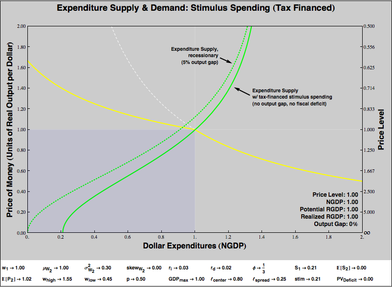
There is a hitch, of course. Our balanced budget is stimulative if and only if spending is increased and balance is accomplished by increasing current taxes. Cutting spending to balance the budget would be contractionary under our framework, while increasing taxes to fund spending is expansionary.

The intuition is pretty straightforward: Consumers divide current wealth between spending and saving. If consumer saving decisions compose to insufficient current spending to avoid recession, the government can preempt those choices by taxing current wealth and spending the entirety of the proceeds.

A few issues and caveats —

• Compare the graph above to the previous graph, where the stimulus spending is not funded by taxes. The X intercepts show how large the government’s spending program must be to eliminate the output gap. Unsurprisingly, government must commit to a great deal more spending to render a funded stimulus effective than it would need to for an unfunded stimulus.
• If the spending program were funded by future period taxes rather than current period taxes, the graph would look nearly identical, given the near-perfect substitutability of present and future money in our model. However, as we discussed above, in the real world, consumers find it expensive or impossible to borrow from the future in recessions, so transferring wealth to current consumers and taxing in the near future to pay for it may be directly expansionary. If that is so, then the scale of government spending required to cover the output gap would be smaller if the spending is paid for out of future taxes rather than out of present taxes.
• If a government commits to large nominal expenditures irrespective of what is to be purchased, indiscriminate spending decisions might degrade the quality and value of current output. If so, effect of the increase on current expenditures might be undone, partially or completely or worse than completely, by a supply-side losses. See “supply and technology shocks” below for an example.

Distributional Effects

Part of my motivation in developing this framework was to come up with a way of conveniently analyzing distributional effects. We can compute different expenditure supply curves for subpopulations of different wealth levels, and “horizontally add” those curves to get the economy-wide expenditure supply. I thought I would easily be able to define some very rough distribution parameter, and show how redistribution affects expenditure supply.

I began with a very strong prior: I believed, and still believe, that the poor are much more likely to spend out of current income than the rich, so that redistribution from rich to poor would increase current expenditures (that is, render the slope of the expenditure supply curve more shallow). To get a quick and dirty take on distribution, I compared two economies, one in which all the wealth was held by a single individual, and a second in which the wealth was equally distributed among many individuals. I expected a shallower curve in the second case.

But that is not what I found, under the utility function above. In fact, it is easy to show that, holding total real wealth (both current and expected future) constant, the expenditure supply curves are identical if the economy contains just one spender (while everyone else starves) or a perfectly equal distribution of wealth. So have I revised my priors?

No, not at all. Instead, I’ve understood deficiencies in my utility function, deficiencies that I think are shared with most utility functions used to build macro models. Why is expenditure supply constant, regardless of distribution? It’s pretty simple really. Under the terms of the model, agents are perfectly forward-looking and all wealth must be spent eventually. Intuitively, we think poor people will spend money today if we put it in their hands because the absolute cost of not spending — going hungry, for example — is large. But, given the structure of my and most macro models, agents don’t evaluate current expenditure against absolute gains in present utility, but against opportunity costs in future utility. If an agent is poor, sure, not eating today has a large cost. But eating today exacts a similarly large cost from the still-poor-me of tomorrow. A rich agent gains little by eating a bit more today, but her cost in future consumption for that benefit is similarly low. Under my utility function, as long as the two agents discount future utility identically, they will make precisely the same tradeoff between expenditures today and expenditures tomorrow. So a poor person, despite starvation, will be just as disinclined to spend current wealth as a rich person. The poor person will balance starvation tomorrow against hunger today, and save some fraction of her wealth. The rich person will balance the pleasures of a bon bon tomorrow against a cookie today, and save precisely the same fraction.

I think this is entirely unrealistic, but what’s interesting is to articulate why. Let’s think about it. In my model, all agents live for precisely two periods, no matter how much or how little they consume. In the real world, insufficient consumption today implies death and zero consumption in the future, regardless of how much a person might have saved. So a realistic model needs some concept of subsistence, such that as present consumption falls and the probability of death increases, the value of future savings is increasingly discounted. More generally and less drastically, future wages in my model are stochastic, but independent of present consumption. But that makes no sense. My ability to earn future wages depends upon my current expenditures. My distribution of future wages is dramatically different if I have a home, decent clothing, a telephone, or an education, than if I do not have these things. Ultimately, I need to add to my consumers’ utility function some notion of investment expenditure that impacts future wealth, rather than restricting the choices to pure consumption and financial savings for interest. And there should not be a single, economy-wide investment return, but each individual’s returns should (usually) be diminishing in wealth. My first dollar of expenditure buys me the ability to survive into tomorrow and enjoy potential future wages; its return is very high. Direct investment of my millionth current dollar might buy me an additional nice suit or make some marginal contribution to a business, but its effect on my future wealth is likely to be small. If I include this sort of direct investment in my model, I think I’d generate the expected relationship between poverty and a bias towards current expenditure. But that’s an exercise I’ve not yet done.

Technology and Real Supply Shocks

The supply side of our economy is graphical represented by the yellow expenditure demand curve. That curve is based on a hyperbola, whose numerator is the capacity of the economy in units of real output. A negative real supply or technology shock yields a recession, without any change in consumers’ willingness to spend:

Note that the output gap is 5%, just like demand-shock recession we’ve illustrated in previous graphs. However, this recession is actually much worse. The real output of our economy has fallen by 13%, not by 5%. The negative supply shock eliminated almost 9% from our potential output. Plus, even though the expenditure supply curve has not changed at all, the shift in the expenditure demand curve pushed the equilibrium onto that curve’s rigid price region, generating an output gap of 5% of our diminished potential output (about 4% of our original output) in addition to the loss of real capacity. In response to a negative supply shock, increasing consumers’ willingness to spend can eliminate the loss of output due to price rigidity, but cannot affect the loss of real capacity:

It’s worth commenting on how the shape of the expenditure demand curve as it shifts in response to a supply shock. By hypothesis, the “kink” in the curve is a function of nominal indebtedness. A firm that requires a dollar of revenue to service its debts doesn’t reduce the price of its total output below a dollar, even if a technology shock diminishes the quantity or quality of that output. So the kink stays where it began, at nominal expenditure of 1.

Yet consumers’ willingness to spend is a depends on the value of real output provided. Holding constant expectations about the future, consumers are less willing to provide that dollar of current expenditure for less or worse stuff. So despite a higher current price level — which you might think would ease the burden of servicing on nominal debt — the diminishment of nominal expenditure occasioned by transiently higher prices (the left-shift of the equilibrium) means that firms have a significantly harder time servicing their debts.

Note that, perhaps counterintuitively, our output gap arises because consumers are optimistic that the real supply shock is temporary. If consumers expect the supply shock were permanent, and therefore that the future price level would rise along with the present price level, a demand effect offsets the supply effect, and the output gap disappears. Consumers become more willing to supply expenditures now because they no longer expect tomorrow’s money to be more valuable than today’s. (The shift in the yellow expenditure demand curve is the real supply shock. The shift in the green expenditure supply curve shows the increase in current spending due to expectations of future high prices.)

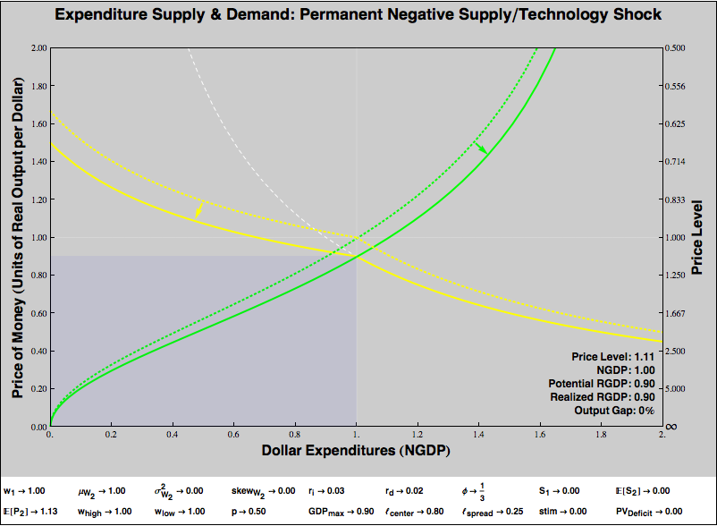
“Stagflation” comes from any sort of negative real supply or technology shock, but is magnified when consumers believe the shock to be temporary!

This is an important difference between demand and real supply side shocks. If consumers’ inflation expectations are “adaptive”, that is, if we learn from experience to predict the future, then for supply shock, changes in expectations help stabilize the current price level and eliminate any output gap. For a demand shock, adaptive expectations about prices are destabilizing. If a demand-driven deflation means we expect future deflation, that diminishes our willingness to spend, which renders our current output gap and deflation even worse. Supply shocks self-heal, demand shocks self-destruct. (Remember, “supply shocks” are shifts in the the expenditure demand curve of our framework; “demand shocks” are shifts in expenditure supply!)

Of course, even if consumers do believe a real shock to be temporary, the output gap can be eliminated by expansionary monetary or fiscal policy. However, no amount of monetary or fiscal policy can undo the real shock. If potential real GDP has fallen by 10%, encouraging people to spend can eliminate the output gap due to price rigidity, but cannot (in a static sense, at least) bring back the lost potential output.

Until the last graph, we’ve considered changes ceteris paribus, adjusting one or two parameters and imagining that all the rest can be held constant. But of course, most of the controversy surrounding proposed policy interventions is about the way in which various changes are interrelated. So, for example, earlier we showed a graph in which stimulus spending eliminated the output gap from a demand shock. However, those who oppose stimulus often argue that poorly targeted government spending will reduce the quality of real output delivered by the economy. Thus, a demand-side remedies will provoke a reduction of real supply. Let’s illustrate that claim:

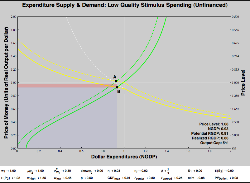
Point A on the graph represents a demand-driven recession, the same recession we graphed in Figure 5. If we left it alone, the economy would face a 5% output gap. That sucks, so we try fiscal stimulus, exactly as we did in Figure 9. Unfortunately, although we successfully shift the expenditure supply curve, poorly targeted government spending leads to suboptimal real production. The expenditure demand curve shifts downward. We end up in a different recession, a worse recession in this example, at Point B.

So what does our analysis say? If we use stimulus spending to counter a recession, will it lead us towards the happy outcome diagrammed in Figure 5 or the terrible outcome diagrammed above? I don’t know. As we said at the outset, our toy model is designed to illustrate possibilities, not to choose among them. But he have learned something about how to consider the question. If government spending is of sufficiently high quality that it doesn’t much reduce the value of aggregate output, then it likely can counter demand-shock recessions. If government spending is of such poor quality that the value of aggregate output is impaired by its psychotic purchaser, than stimulus spending may prove badly counterproductive. People’s views on the quality of government expenditures tend to correlate with tiresome political affiliations. My own view is that we have free will, collectively as well as individually, that governments sometimes do deploy resources wisely, but sometimes they make choices that are awful and corrupt. Our work is not to estimate the odds, but to shape the context in which government acts so that it is likely to act well.

If you think this story argue for monetary expansion as opposed to fiscal stimulus, think again. We can tell almost exactly the same story. Expansionary monetary policy, like government spending, increases our aggregate propensity to spend. But who says it has no effect on the production side of the economy? My own view, with the Austrians and other cranks, is that stimulating demand via low interest rates does cripple real supply over time, in part by favoring producers of durable goods, but more insidiously by altering the incentives of holders of financial assets, who diversify to capture monetary policy subsidies rather than discriminate between worthy and unworthy enterprises. I would rather take my chances with more transparent (if transparently corrupt) fiscal policy than with status quo monetary policy.

But that’s just me. The framework we’ve set up can illustrate happy and tragic stories, for both monetary and fiscal interventions. Further, if we come up with models that specify relationships between the parameters, or between the demand side and the production side of the economy, we can illustrate those models with the same sort of graphs we’ve shown here.

We’ve been working with a discrete, two period toy model. However, that’s limiting. For example, if poor government spending harms the supply side of the economy, the effect may not be simultaneous. We’ve crammed several non-instantaneous effects into “Period 1”. But we can draw graphs like this as “snapshots” of models that evolve over time. We can even combine graphs into annoying little movies to watch the economy evolve under various scenarios.

This has been a long exercise, and I’m grateful to readers who’ve made it this far. I’ve learned a lot from playing around with these graphs, but I’ve no idea whether doing so will help others. I hope so!

---

If you haven’t yet, do try playing around with the interactive graphs here. (You’ll need to install the Mathematica plug-in.)

RSJ, whose excellent blog is windyanabasis, takes issue with my claim that financial leverage is a source of sticky prices. Not only that, but he’s performed an impressive experiment to test and disprove the hypothesis. Check it out.

I am not persuaded that I am wrong, for reasons that I describe in a lengthy comment. But I am hardly an impartial reviewer. What do you think?

Update: RSJ has updated his experiment in response to some of my comments.

In Keynesian / quasi-monetarist of explanations of depression, sticky prices play an essential role. If prices were not sticky, a deficiency of expenditure would just lead to a reduction of the price level, and nothing very bad would happen. There are (at least) two channels by which sticky prices can harm production:

1. Sticky relative prices distort patterns of economic activity, preventing the economy from achieving the optimal level of production. Following a sharp change in nominal expenditure, the sluggishness with which some prices adjust leaves activity badly distorted, and so observed real production falls relative to the expenditure-stabilized trend.
2. Sticky absolute prices allow changes in nominal expenditure to affect levels of economic activity more directly. Suppose we set all relative prices correctly, and then fix them in stone. Now, if we scale up the willingness of all agents to part with money, we might not observe a decline in aggregate production, but markets would fail to clear and we would observe shortages. If we scale down aggregate expenditure, we would observe a glut of capacity and a fall in production (as measured by transactions).

I’m interested here in the second channel. [1] Except under politically imposed price controls, we rarely observe what absolute price-stickiness would predict in an expenditure boom — production at capacity but shortages at offered prices. The relevant case is asymmetrical. Absolute prices adjust upward easily, but they are “sticky downward”. They do not fall.

A while back I had a post that described the price of extinguishing old debt as “the stickiest price”. After a wonderful comment exchange with Nick Rowe and others, we came, I think, to some agreement that sticky nominal debt contracts were both like and unlike sticky goods prices in important ways. However, I’ve recently come to think that, besides the direct but distinct distortions associated with rigid nominal debt, indebtedness might be an important source of downward stickiness in the prices of goods and services.

The argument is a form of Pascal’s wager. Suppose that I own a firm which generally operates at capacity. The firm is leveraged in the expectation of achieving a certain level of nominal income, out of which my debt will be serviced. Should I fail to service my debt, I will face outcomes that are very dire. Perhaps my firm will be out of business, perhaps I will have to surrender the firm to creditors. Perhaps I’ll manage to squeak by after a very radical downsizing that allows me to service my debts but destroys the long-term value of the firm. Let’s refer to any of these catastrophes as “bankruptcy”.

Suppose there is a shock to nominal demand, and people become less willing to part with money. I have two choices. I can cut prices to maintain my expected volume of sales, or I can leave prices alone. In the first case, I condemn myself to bankruptcy with certainty. I was already operating at capacity, so there is no hope that an increase in volume will save my bacon if I reduce prices.

If I do not cut my prices, my expected level of sales will fall due to the recession. On average, I will still be bankrupt. But I could get lucky. In any economic environment, sales are a fickle random variable. It is possible, if I stick with my old prices, that sales will prove robust despite the dowturn. So the rational thing for me to do is to refuse to adjust my prices and hope for the best.

Now this is a perverse outcome, from an economic perspective. Considered without regard to financing, my firm fails to maximize expected profits by failing to adjust its pricing. It instead maximizes the value of the right tail of the profit distribution, because as the owner of a leveraged firm, the right tail of the distribution is all that I have claim to. Not reducing prices is a form of screwing creditors, but I don’t care. As the owner of a highly leveraged firm operating near capacity, I will be disinclined to reduce prices.

This tale of an overleveraged entrepreneur would be insignificant, if it were an idiosyncratic occurrence. One overextended entrepreneur might refuse, but her less leveraged competitors would cut prices, and observed market prices would fall. But suppose our entrepreneur is in an industry where intense leverage is the norm. As Hyman Minsky famously pointed out, if an industry is competitive and at least some players are not foresighted about risk, levering up in good times ceases to be optional. More levered firms gain a cost-of-capital advantage that permits them to undercut financially conservative rivals over what may be prolonged periods of tranquility. So we might expect to competitive forces to drive whole industries into similar capital structures. And empirically we do find this — firms in general choose wide varieties of capital structures, but within industries, capital structures are more alike.

In highly leveraged industries then, we’d expect downward price stickiness. Following a negative shock to nominal expenditures, we would observe production losses, but not in the form of evenly distributed cutbacks. Instead, some firms would seem to thrive despite the weather, while others are forced into bankruptcy. Perhaps the firms that survive would be the “best” firms, and certainly differences in quality and ex ante leverage would affect the distribution of outcomes. But even among perfectly identical firms, if the distribution of sales is stochastic, we’d expect “consolidation” to occur. Firms that are lucky early in a depression survive. It gets easier to stay lucky as time goes on. The failure of competitors eliminates supply, helping to support your sticky price (which becomes less sticky as you retain earnings to delever).

From a macroeconomic perspective, this account suggests that, even putting aside systemic fragilities introduced by cascading bankruptcies and financial accelerators running in reverse, financial leverage leaves an economy vulnerable to depression through a price rigidity channel. This strikes me as relevant to our current situation. Policymakers have effectively guaranteed the debt of highly interconnected borrowers and successfully eliminated the threat of cascading defaults. But if my account is correct, reducing leverage at “Main Street” firms may be at least as important as ensuring the stability of interconnected financials. Policymakers have put tremendous effort into ensuring the continuous availability of credit to firms that wish to expand. But promoting debt-financed expansion may be self-defeating, if it reduces the ability of the economy to adapt to fluctuations in nominal expenditure by making prices sticky. [2]

---

Notes:

1. This will be an intramural point. Footnote 2 is more interesting.

   I think that explanations of the business cycle based on relative price stickiness ought not be classified as Keynesian or monetarist at all. Relative price stickiness is really a recalculation story of the sort favored by Arnold Kling (and to which I am also sympathetic). If you think of markets as calculators of equilibria, and that after a large shock computing a new equilibrium takes time, then there must be some sort of friction that prevents the computation from being instantaneous. Sticky prices offer one plausible source of friction.

   I won’t speak for Kling, but I think that some proponents of recalculation-ish theories would object to this characterization, because they view economic calculation as something deeper than a rejiggering of relative prices. They’d focus instead on inspired entrepreneurship, creative destruction, entirely new practices and products. I agree with all that, but when making up models we do have to reduce a variegated and multicolored world to symbols, and modeling recalculation as a laborious price vector computation is more expressive than it first appears. For example, we can imagine a space of potential new products whose prices begin at infinity and adjust downward with difficulty, as we learn by doing or as a stochastic function of entrepreneur effort.

   It might seem odd to expel relative-price-stickiness-based explanations from the Keynesian pantheon. After all, aren’t New Keynesian models almost defined by incorporation of relative price stickiness? Well yes, and they use relative price-stickiness to achieve monetary non-neutrality. However, at risk of stepping on toes (which is really not my intention), I think that by construction New Keynesian models are poorly suited to the analysis of extreme business cycles. New Keynesian models, like their Real Business Cycle progenitors, are usually characterized in log-linear approximation around a long-run equilibrium. Even if we believe the models to be perfectly correct, the conclusions we draw from log-linear approximations become less and less reliable as variables depart from equilibrium values. Log linearized models, if they are useful, are useful at describing near-equilibrium dynamics. If extreme business cycles involve severe departures from the presumed equilibria, or worse yet, if they involve multiple equilibria so that the economy might be durably drawn away from the presumed steady state, common New Keynesian models just aren’t helpful. To invoke Hyman Minsky again (via Steve Keen), if you want to answer questions about extreme business cycles

   it is necessary to have an economic theory which makes great depressions one of the possible states in which our… economy can find itself.

   Perhaps I am overharsh. I am certainly no expert on New Keynesian macro, and I’d be delighted to learn that I am wrong. But the New Keynesian models I have encountered simply don’t live up to Minsky’s very sensible criterion. Monetarist and Old Keynesian models, though hydraulic and not-microfounded they may be, incorporate in their design the possibility of durable and severe depressions. [ back ]

2. The story I’ve told isn’t particularly novel. It complements commonplace accounts of why unemployment occurs in depressions. In theory, firms could simply cut employee hours and wages rather than fire people in response to a downturn. But they don’t. Employment adjusts on the “extensive” margin of layoffs much less than it adjusts on the “intensive” margin of reducing work or pay. This is often attributed to employee morale. It is better, the story goes, to have a small workforce of happy people than a big workforce of bitter people.

   But consider the same situation from employees’ perspective. Families are often highly leveraged. Even when they are not explicitly in debt, many families take on operating leverage. That is, for many families, the fixed costs of ordinary living (e.g. rent, day care, food) approach their total household income. With high leverage (whether explicit debt or operating leverage), a reduction of wages and hours translates quickly to financial and personal crisis, and ultimately to a disruptive reorganization of living arrangements. A cutback in wages and hours may leave families unable to afford their mortgage or their rent, and force a move to less desirable digs or “doubling up” with family, usually after a lot of confusion and juggling and bills and shame and collection agencies.

   Getting fired will do all that too, of course. But if firms hold wages steady and cut back by firing workers, then some workers will avoid the reorganization entirely. When firms cut wages or hours, all highly leveraged workers must reorganize. If the severity of crisis is not so different for those who are fired versus those who see pay cuts (a big if), then workers rationally prefer a layoff lottery to universal pay cuts. Their reasoning would be identical to that of leveraged firms who hold prices steady and take their chances.

   So firms find layoff lotteries to be better ex ante, because employees prefer them, and ex post because only the happy winners remain with the firm. A perennial suggestion among reformers is that we substitute some form of work-sharing for cyclical unemployment, so that the burden of downturns is evenly shared instead of falling disproportionately on an unlucky few. That sort of reform only makes sense when household leverage is generally modest. [ back ]

Ezra Klein, Karl Smith, and Ryan Avent today debate the merits and demerits of muddling though vs “grand bargains” and bold solutions. Here’s Smith, insightful as always:

The opportunity to muddle through is a gift. It allows one to make changes at the margin, to monitor their effects and to update accordingly. It allows us to avoid massive often useless sacrifice. It allows our knowledge, understanding and resources to race ahead opening up new ways to deal with our problems… We don’t always have that opportunity. Sometimes we are forced to deal with things in a big way. Indeed, this is much of what we mean by crisis. However, you don’t want to avoid an externally inflicted crisis by creating a self-inflicted one. If you have a chance to make your way with adjustments at the margin, take it.

I think this is right, and important. But even true words can lead us astray if we are not careful. To say that muddling through is a gift because it permits certain advantages can mutate into a case for incrementalism where there are clear disadvantages.

Further, which changes constitute “adjustment” and which would be disruptive are themselves contested. Consider Scott Sumner‘s view of the world. Sumner claims that the stance of monetary policy, when properly defined, turned sharply contractionary in 2008. However, what Sumner would have proposed in order to “stay the course” would have seemed bold and radical to status quo central bankers. Generally, what constitutes measured and incremental changes and what constitutes a sharp turn gets defined according the the conventions of dominant interests. Consider the TARP vs bank nationalization debate. The case against nationalization was often made on grounds of continuity and nondisruption, and that certainly reflects the perspectives of people inside the banking system and the Treasury department. And yet to me and many others like me, the no-accountability/no-more-Lehmans policy regime that was crystallized as TARP represents a wrenching and violent alteration of previously settled social arrangements.

Today’s conversation began with US fiscal policy. Klein tells us

The wish for a grand bargain that’ll take care of the deficit all at once is probably just that: a wish. The likelier outcome is a slew of deficit-reduction measures passed over the next decade or so. That’s even truer for health-care spending, which is both the biggest fiscal problem we face and the one that most requires a decades-long process of trial-and-error in which we test out new ways of delivering care, of paying for care, of separating useful treatments from useless ones and of modernizing the sector’s IT infrastructure.

Overall, this seems sensible. There is a problem, but we won’t hubristically predetermine a 30 year plan,. We’ll make small adjustments in real-time until the problem is solved. That sounds wise.

But is it true? Is that how US fiscal issues are likely to play out? I don’t think so. I’d bet on one of the following three scenarios:

1. We will experience a boom and/or create technical efficiencies in health care delivery such that the US fiscal trajectory seems to stabilize on its own.
2. The US fiscal situation will fail to durably stabilize at anywhere near the levels we now deem reasonable, but nothing catastrophic will happen. The MMT-ers will turn out to be right that any inflation or yield pressure associated with a growing stock of public debt will prove manageable in real time. It will feel like we are muddling through perpetually, but nothing bad will ever come of it.
3. A crisis will force bold changes on the political system. This might take many forms — an inflation, a sharp spike in bond yields, a disruptive depreciation of the dollar, popular revolt against the distributional effects of fiscal largesse, etc.

At the moment, Klein’s scenario seems plausible. After all, despite elevated chronic unemployment — which in our society constitutes almost unthinkably severe human tragedy — we are making genuflections towards deficit reduction. Surely this means we are committed, and bit by bit we will adjust. Right?

No. For better or for worse, we are not adjusting. The small changes our political system proves capable of are promises of future chastity and cuts that disproportionately harm the disenfranchised. Historical experience suggests that even this degree of restraint depends upon an ephemeral configuration of political authority — a Democratic president, a Congress divided or Republican. There is little evidence that our government is capable of adjusting, incrementally but intelligently. It follows paths of least resistance and responds to crises. That might work out all right, or it might lead us to catastrophe.

So is it wise to muddle through? I think we all can agree that not all paths of least resistance end up in places one would wish to go. At the same time, Karl Smith is still wise. Sharp, bold changes are ipso facto crises, and there’s no sense creating pain willy-nilly to deal boldly with inexhaustible phantoms.

So what’s the right strategy? I’m not sure, but I’ll tell you what I used to think. I used to think that the right strategy was to muddle through in a context created by sophisticated financial markets. Human beings, as individuals and as policymakers, have limited information and are prone to flawed choices. Markets aggregate the information and foresight of millions, weighted by confidence expensively signaled via degrees of financial risk assumed. Such markets would always be current, would produces prices reflective of the best available information at any point in time, and would be forward looking. Markets would ensure that, on the path of least resistance, peoples’ incentives would be to make smart adjustments in real-time. Muddling through under these circumstances would leave us where Smith suggests: With “knowledge, understanding and resources…opening up new ways to deal with our problems…[we’d make our] way with adjustments at the margin.”

I think that this view, once my view, is now completely discredited. Financial markets, as they exist in the world we live in, have proven liable to catastrophic and foreseeable mistakes. The instruments we trade hide information and prevent adjustments as frequently as they reveal and promote them. Plausible mechanisms of self-correction have been weakened rather than strengthened during the crisis, so we can expect even poorer performance looking forward. Our financial institutions are best understood as means by which certain groups within our society protect and perpetuate themselves, and as mechanisms by which covert prerequisites of stability are maintained. Of course markets were never going to be perfect — no human institution is. But existing market institutions have fallen in my estimation from “good enough, the best we’ve got” to “incompetent and hopelessly corrupt”.

Absent some context that shapes incentives and links muddling through with intelligent adjustment, accepting muddling as a default position is unsatisfactory. It becomes a means of drifting towards hazards unknown and an excuse for attending to the interests of the powerful. The alternative of bold, flawed, improvisations is also unattractive. The choice between moldy bread and rancid stew is best made on a case-by-case basis, with a lot of unscientific sniffing.

The only way out is to recreate some context in which we’ve reason to expect our muddling will be smartly shaped. Our existing political and financial systems strike me as a poor place to start, but here we are. In the end, I’d like to agree with Karl Smith about the virtues of muddling through. But it all hangs on the quality of the muddling.