
Persnickety followups on inequality and demand
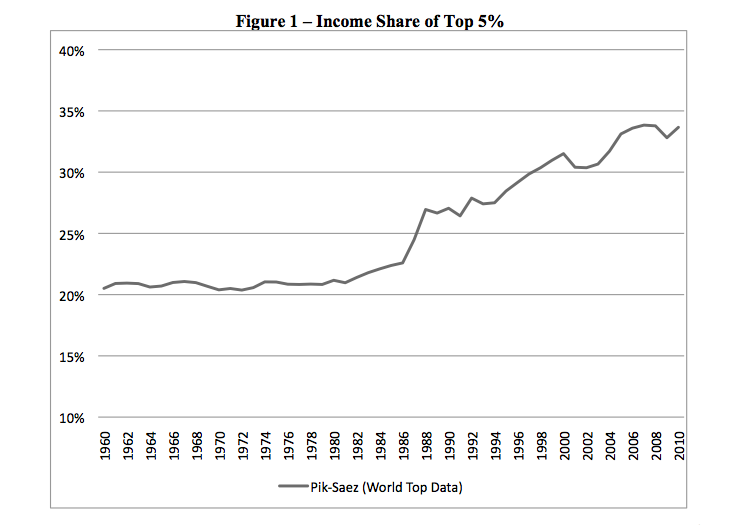
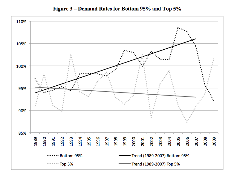
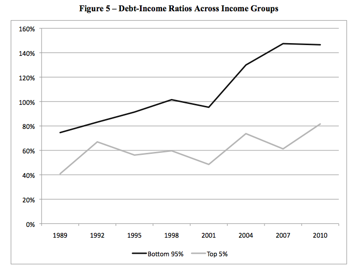
Teaser: The following graphs are from “Inequality and Household Finance During the Consumer Age“, by Barry Cynamon and Steven Fazzari. “Demand rates” are expressed as fractions of “spendable income”. There’s more on this paper at the end of the post.
I am always outclassed by my correspondents and commenters. The previous post on inequality and demand was no exception. I want to follow up on a few scattered bits of that conversation. I apologize as always for all the great writing, in comment threads and in e-mails, that I fail to respond to.
First, I want to make a methodological point. Several commenters (e.g. beowulf, JKH, Mark Sadowski) point to discrepencies between measures of income and saving used by various empirical studies and those used in national accounting statements (e.g. NIPA). In particular, there is the question of whether unspent capital gains (realized or unrealized) should count as saving. NIPA accounts quite properly do not treat capital gains as income.
But what is proper in one context is not proper in another. NIPA accounts attempt to characterize the production, consumption, and investment of real resources in the consolidated aggregate economy. A capital gain represents a revaluation of an existing resource, not a new resource, and so properly should not be treated as income.
However, when we are studying distribution, what we are after is the relative capacity of different groups to command use of production. We must divide the economy into subgroups of some sort, and analyze interrelated dynamics of those subgroups’ accounts. Capital gains don’t represent changes in aggregate production, but they do shift the relative ability of different groups to appropriate that output when they wish to. When studying the aggregate economy, capital gains should be ignored or netted-out. But when studying distribution — “who owns what” — capital gains, as well as the dissaving or borrowing that funds those gains, are a critical part of the story. Research on how the distribution of household income affects consumption absolutely should include capital gains. There are details we can argue over. Unencumbered, realized capital gains should qualify almost certainly as income. Gains from favorable appraisal of an illiquid asset probably should not. Unrealized gains from liquid or hypothecable assets (stocks, real estate) are shades of gray. There is nothing usual about shades of gray. All spheres of accounting require estimation and judgment calls. Business accountants learn very quickly that simple ideas like “revenue” and “earnings” are impossible to pin down in a universally satisfactory way.
Similar issues arise in interpreting the excellent work of J.W. Mason and Arjun Jayadev on household debt dynamics, to which Mark Sadowski points in the comments. Mason and Jayadev decompose the evolution of the United States’ household sector’s debt-to-income ratio, breaking down changes into combinations of new borrowing and interest obligations (which increase debt-to-income) plus inflation and income growth (which decrease debt-to-income). It’s a wonderful, fascinating paper. If you’ve not done so already, I strongly recommend that you give it a read. It’s accessible; much of the tale is told in graphs. (A summary is available at Rortybomb, but you want to study especially Figure 7 of the original paper.)
One of Mason and Jayadev’s most interesting discoveries is that the period since the 1980s has been an “Era of Adverse Debt Dynamics”, a time during which household debt-to-income increased because of reductions in inflation, low income growth and a high effective interest rate on outstanding debt. [1] For most of the period from 1980 to 2000, the aggregate US household sector was not taking on new debt. Household sector debt-to-income deteriorated despite net paydown of imputed principal, because of adverse debt dynamics.
So, can a theory that claims borrowing by lower-income households supported demand over the same period possibly be right? Yes, it can. At any given time, some groups of people are repaying debt and others are taking it on. If, say, high income boomers are paying off their mortgages faster than low-income renters are borrowing to consume, new borrowing in aggregate will be negative even while new borrowing by poorer groups supports demand. (Remember how back at the turn of the millennium we were marveling over the “democratization of credit“?)
As always, when studying distributional questions, aggregate data is of limited use. That’s not to say that there is no information in aggregate data. It’s definitely more comfortable to tell the borrowed demand story about the 2000s, when, Mason and Jayadev show us, aggregated households were dramatically expanding their borrowing. But what we really want is research that disentagles the behavior of wealthy and nonwealthy households.
A working paper by Barry Cynamon and Steven Fazzari does just that. It tells a story quite similar to my take in the previous post, but backs that up with disaggregated data. The three graphs at the top of this post summarize the evidence, but of course you should read the whole thing. There is stuff to quibble over. But the paper is an excellent start.
I’ll end all this with an excerpt from the Cynamon and Fazzari paper that I think is very right. It addresses the question of why individuals would undermine their own solvency in ways that sustain aggregate spending:
It is difficult for standard models, most notably the life cycle model, to account for the long decline in the saving rate starting in the early 1980s. A multitude of economists propose explanations including wealth effects, permanent income hypothesis (high expected income) effect, and demographics, but along with many researchers we find those explanations unsatisfying. We argue that the decline in the saving rate can best be understood by recognizing the important role of uncertainty in household decision making and the powerful influence of the reference groups that to which those household decision makers turn for guidance. We propose that households develop an identity over time that helps them make consumption decisions by informing them about the consumption bundle that is normal.9 We define the consumption norm as the standard of consumption an individual considers normal based on his or her identity (Cynamon and Fazzari, 2008, 2012a). The household decision makers weigh two questions most heavily in making consumption and financial decisions. First, they ask “Is this something a person like me would own (durable good), consume (nondurable good), or hold (asset)?” Second, they ask “If I attempt to purchase this good or asset right now, do I have the means necessary to complete the transaction?” Increasing access to credit impacts consumption decisions by increasing the rate of positive responses to the second question directly, and also by increasing the rate of positive responses to the first question indirectly as greater access to credit among households in one’s reference group raises the consumption norm of the group. Rising income inequality also tends to exert upward pressure on consumption norms as each person is more likely to see aspects of costlier lifestyles displayed by others with more money.
People will put up with almost anything to live the sort of life their coworkers and friends, parents and children, consider “normal”. Over the last 40 years, for very many Americans, normal has grown increasingly unaffordable. And that created fantastic opportunities in finance.
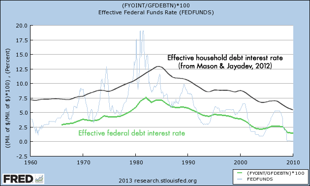
[1] Mark Sadowski suggests that the stubbornly high effective interest rates reported by Mason and Jayadev are inconsistent with a claim that the secular decline in interest rates was used to goose demand. But that’s not quite right — it amounts to a confusion of average and marginal rates. At any given moment, most household sector debt was contracted some time ago. The effective interest rate faced by the household sector is an average of rates on all debt outstanding, and so lags headline “spot” interest rates. But incentives to borrow are shaped by interest rates currently available rather than rates on debt already contracted. Falling interest rates can increase individual households’ willingness to borrow much more quickly than they alter the aggregated sector’s effective rate.
In my first encounter with the Mason and Jayadev paper, I thought I saw in the stubbornly high effective rates evidence of a rotation from more-creditworthy to less creditworthy borrowers. (See comments here.) I’ve looked into that a bit more, and the evidence is not compelling: the stubbornly slow decline in household sector interest rates pretty closely mirrors the slow decline in the effective interest rate of the credit-risk-free Federal government. There’s a hint of spread expansion in the late 1990s, but nothing to persuade a skeptic.
Waldman: People will put up with almost anything to live the sort of life their coworkers and friends, parents and children, consider “normal”. Over the last 40 years, for very many Americans, normal has grown increasingly unaffordable. And that created fantastic opportunities in finance.
—————
Keynes answered this question long ago from the perspective of the long-term investor in the type of investment, but the reasoning is pretty much the same in terms of the level of consumption versus saving.
John Maynard Keynes
The General Theory of Employment, Interest and Money
Chapter 12. The State of Long-Term Expectation
Part V
Finally it is the long-term investor, he who most promotes the public interest, who will in practice come in for most criticism, wherever investment funds are managed by committees or boards or banks.[4] For it is in the essence of his behaviour that he should be eccentric, unconventional and rash in the eyes of average opinion. If he is successful, that will only confirm the general belief in his rashness; and if in the short run he is unsuccessful, which is very likely, he will not receive much mercy. Worldly wisdom teaches that it is better for reputation to fail conventionally than to succeed unconventionally.
February 12th, 2013 at 7:53 pm PST
link
a very tangential point – there are lots of models around in which people derive utility relative consumption (consumer more or less than their peers).
Academics are frequently baffled by the desire to own a Porsche, for example, (the idea that people might simply really like Porsches not being taken seriously) and rationalise it by saying that Porsche owners derive pleasure from having a better car than everybody else, rather than from the Porsche itself. Now I’m sure some people gain some pleasure from being the object of envy, but I’ve always disliked this “conspicuous consumption” model because it’s mean spirited and construes rich people with nice things as pretty horrible, and I suspect functions mainly to allow people without Porsches to feel morally superior to those with.
But I really like these models in which we judge ourselves based on some peer group based sense of normality, or relative to some sense of identity that we construct from our peers. It makes sense to me if we are programmed to feel happy when things are going better than we could expect, and unhappy when things are going worse. But we don’t know what we ought to expect, so we use a reference group to form an idea of what we ought to be comparing our experiences too. I think this is just a different interpretation of a relative consumption model, with a more generous interpretation of happy successful people. I like to think that I would be happy if my life turned out to be unexpectedly successful, because I’d feel blessed by good fortune, not because I’d directly derive pleasure from the gap between myself and those less fortunate.
[full disclosure: my car cost $2000, but I do have a rich friend with a Porsche and I think he just likes it for its own sake]
February 13th, 2013 at 6:29 am PST
link
[…] See full story on interfluidity.com […]
February 13th, 2013 at 2:18 pm PST
link
A detailed post I left, has been lost in the ether… In summary:
1) If you are really worried about how much money people have after paying their debt, why not look at household debt service ratio? It is a much more elegant statistic than raw debt/income. http://research.stlouisfed.org/fred2/series/TDSP
2) The type of debt is important. From the household debt tables, we can see that the composition of debt has changed in the past couple decades. It used to be 75%/25% mortgage/consumer. It is now 80%/20% mortgage/consumer.
Table D.3: http://www.federalreserve.gov/releases/z1/Current/z1.pdf
3) To go from 80 to 140 units of debt (%/income or otherwise), while the composition of that debt changed from 75%/25% to 80%/20%. It can be shown that:
Total debt increased 75% (from 80 to 140).
Mortgage debt is 85% of this increase.
Consumer debt (cars, plastic, etc.) is 15% of this increase.
We are more indebetted, but the new debt is overwhelmingly mortgage debt.
4) While most of the increase of debt has been mortgage debt, the interest rates on mortgage debt has been cut by 60%+. Cutting mortgage rates from 10% to 3.5% will halve your mortgage payment, on a $100k principle.
http://research.stlouisfed.org/fred2/series/MORTG
———-
While the bottom 95% have more debt/income. It costs them less to service this debt, and therefore people have more disposable income.
Debt/income is meaningless.
If we look an important statistic like disposable income after servicing your debts, then we see a direct correlation to the “demand rate” curve you present. Demand went up WITH increased debt payments. Demand is now recessing ALONG WITH lower debt servicing payments.
This is completely opposite of what you are attempting to show. (Note that the data I present is aggregate and not “by the classes” you present.) (And the data do not show people paying off debt in excess of the servicing requirment.)
February 13th, 2013 at 2:35 pm PST
link
While I’m absorbing this exercise in persnicketyness, allow me to share some (very) rough disaggregated estimates I already made a few weeks ago using Fisher dynamics and data from Edward Wolff. (I came to somewhat different conclusions.):
http://www.levyinstitute.org/pubs/wp_589.pdf
According to Table 7 the top 1% have seen their leverage ratio fall from 86.8% to 39.4% of income and the middle 60% have seen their leverage ratio increase from 66.9% to 156.7% of income from 1983 to 2007. According to Table 4 the top 1% have seen their real income increase by 127.2% and the middle 20% by 7.7% from 1982-2006. I’m going to make the simplifying assumption that the figure for the median is the same as for the middle 20% and middle 60% above. I’m also going to assume that the top 1% and median are the same households at the beginning (1982/83) as at end (2006/2007).
To make the calculations easier to explain I’m going to make some simplifying approximations. The “Fisher effect” is approximately equal to the real interest rate minus the growth rate of real disposable income. (It is also approximately equal to nominal interest minus the growth rate of nominal income.) And, finally, average growth in leverage per year is approximately equal to the Fisher effect plus the primary deficit (or minus the primary surplus).
From 1983-2007 real interest was approximately 5.5% (see Mason and Jayadev). The the growth rate of real income was 3.5% for the top 1% and 0.3% for the median. Thus the Fisher effect is approximately 2.0% and 5.2% for the top 1% and the median respectively. The average growth in leverage per year for the top 1% and the median is (-2.0%) and 3.7% respectively. So, finally, the primary surplus for the top 1% and the median is approximately 4.0% and 1.5% on average over the entire period 1983-2007 respectively.
Thus the large difference in the evolution of leverage can be easily be explained without resorting to nonexistent credit flows. It very likely owes much more to the large difference in the rate of growth in real disposable income than it does to differences in the primary deficit.
February 13th, 2013 at 5:25 pm PST
link
“But what is proper in one context is not proper in another. NIPA accounts attempt to characterize the production, consumption, and investment of real resources in the consolidated aggregate economy. A capital gain represents a revaluation of an existing resource, not a new resource, and so properly should not be treated as income.
However, when we are studying distribution, what we are after is the relative capacity of different groups to command use of production. We must divide the economy into subgroups of some sort, and analyze interrelated dynamics of those subgroups’ accounts. Capital gains don’t represent changes in aggregate production, but they do shift the relative ability of different groups to appropriate that output when they wish to. When studying the aggregate economy, capital gains should be ignored or netted-out. But when studying distribution — “who owns what” — capital gains, as well as the dissaving or borrowing that funds those gains, are a critical part of the story. Research on how the distribution of household income affects consumption absolutely should include capital gains.”
Actually, I couldn’t possibly disagree more. We’re talking about the the “underconsumption” hypothesis, basically that the rich spend too little of their income. That is, the rich are spending too little of their share of new resources. But since capital gains are not part of the flow of new resources it makes no sense to include them when trying to estimate how much the rich are contributing to “underconsumption” of new resources.
The claim that capital gains reflect relative ability of different groups to appropriate output when they wish to also seems highly incorrect to me. First of all capital gains are existing resources, not new output. Secondly, capital gains realizations are highly influenced by tax rates, particularly changes in tax rates. A paper by Slemrod demonstrating this may be found here:
http://www.nber.org/papers/w3237.pdf
This underscores the fact that capital gains realizations are almost always voluntary and tell us much more about the desire of the rich to avoid taxes than they do about the changing ability of the rich to tap into their existing stock of resources. Capital gains are more an IRS accounting exercise than anything that has implications for the real economy.
February 13th, 2013 at 6:37 pm PST
link
“Mark Sadowski suggests that the stubbornly high effective interest rates reported by Mason and Jayadev are inconsistent with a claim that the secular decline in interest rates was used to goose demand. But that’s not quite right — it amounts to a confusion of average and marginal rates. At any given moment, most household sector debt was contracted some time ago. The effective interest rate faced by the household sector is an average of rates on all debt outstanding, and so lags headline “spot” interest rates. But incentives to borrow are shaped by interest rates currently available rather than rates on debt already contracted. Falling interest rates can increase individual households’ willingness to borrow much more quickly than they alter the aggregated sector’s effective rate.”
This is true. However the original issue was not nominal interest rates, but real interest rates. Inflation has also trended downward over this time period. One way of trying to account for both effects is to look at the current real rate of interest on mortgage loans, which of course comprise approximately three quarters of household sector debt. Here is the 30-year conventional mortgage rate, the PCE deflator and their difference from 1972 through 2012:
http://research.stlouisfed.org/fred2/graph/?graph_id=107186&category_id=0
Borrowing the division in time periods from Mason and Jayadev we find that the real mortgage rate averaged 2.2% from 1972 through 1980, 6.8% from 1981 through 1999, 4.2% from 2000 through 2006 and 3.0% from 2007 through 2012. So yes, looking at current real rates, we do see a downward trend, but note that the average real mortgage rate is higher in each of the three periods when inequality has been increasing than in the 1970s when inequality was at or near a trough by most measures.
February 13th, 2013 at 7:34 pm PST
link
Mark A. Sadowski, is it really true to say that capital gains are not part of the flow of new real resources? The value of land or art or whatever increases in line with what people can afford to pay for it. What they can afford to pay for it depends on the flow of new real resources and expansion of credit (and credit expansion presumably eventually also is limited by the flow of new real resources).
If you owned a valuable painting since 1939, you would now be able to exchange it for say a lot more coffee cups than when you got it. That painting value was rooted in and expanded along with the real economy.
Imagine two people, one owns Berkshire Hathaway stock and the other owns stocks owned by Berkshire Hathaway. The first will get unrealized capital gains but no income, the second will get dividends and perhaps reinvest those to replicate Berkshire Hathaway. Are you saying one is doing more “saving” than the other?
February 14th, 2013 at 4:39 am PST
link
Mark A. Sadowski, imagine an extreme case where all of the land and all of the banks are own by a few oligarchs. They have bought the land with loans from the banks such that all of the rent they get goes to pay the interest on the loans. The banks retain earnings such that minimal dividends are paid. Only a tiny fraction of the land rent ends up as income for the oligarchs. All of the rest of it ends up as capital gains for the oligarchs (land prices and bank stock prices). The oligarchs do spend all of the remaining income but can you really say that the oligarchs are not causing a high saving rate and so under-consumption across the economy? The rent paid by the “little people” is a big chunk of the whole economy.
February 14th, 2013 at 5:28 am PST
link
Thanks as usual for the food for thought.
I just want to point out that the thing with unrealized capital gains is not so simple. There is a good case to consider some capital gains as “income” for income accounting purposes, and there is also a good case to exclude some unrealized capital gains for distribution analysis purposes.
For instance, suppose you have an apple tree that produces 50 apples per year and is worth, say, $100. Now through your labor of love you increase the productivity of this tree to 100 apples per year. You have a $100 unrealized capital gain. This is not, however, just the revaluation of an existing resource.
A different, less clear-cut example is the following. You own a house in the periphery of Brooklyn. The City of New York builds a new express subway line and suddenly you can be from your apartment to Times Square in 30 minutes. (Before it was 90). The value of your house increases by 200%. In this case the unrealized capital gain simply represents a spillover of value that the owner of the subway line has declined to appropriate. What created value is the subway line (a real resource increase) but its value shows up in the property values of its users. Here again you have an unrealized capital gain that is directly linked to a new resource.
Finally, for distributional reasons, try to think what could happen to the unrealized capital gains of long-time Microsoft stockholders if Bill Gates (or his foundation) suddenly decided to sell everything on the open market. It’s not obvious that $1 of unrealized capital gains can command $1 of resources valued at the pre-realization prices.
February 14th, 2013 at 8:25 am PST
link
I’ve had a chance to scan some of the work of Barry Cynamon and Steven Fazzari.
In some ways this working paper looks at household sector finances over this period from the flip side of Mason and Jayadev. Whereas Mason and Jayadev tackle income, Cynamon and Fazzari look at expenditures. Both papers make adjustments to the treatment of housing, Mason and Jayadev subtracting imputed rent, property taxes etc. from disposable income, and Cynamon and Fazzari subtracting imputed rent and adding residential investment etc. from/to personal consumption.
Mason and Jayadev note that their adjustment is necessary because the NIPA treatment of housing is inconsistent with the general NIPA convention of not including non-market transactions. Presumably Cynamon and Fazzari are making similar adjustments for similar reasons. But they don’t just stop at housing. As an earlier paper notes (Section I Part B):
“These adjustments lead us to new definitions of household demand, household income, transfer payments made by households (largely rent and interest payments), and even a new measure of GDP. In what follows, we refer to these new measures as “adjusted” to distinguish them from the standard measures in the NIPA data.”
http://artsci.wustl.edu/~ec448sf/cyn-fazz_inequal.pdf
They make so many adjustments without clear exposition of what they are doing that in my opinion it is essentially impossible to reproduce their results.
Of more interest in this context (at least to me) is their treatment of savings. In my original series of comments (on your previous post) I cited the work of Maki and Palumbo in claiming that there was evidence that NIPA consistent savings rates show that, at least in 2000, savings rates actually declined as income increased. Well on page 7 they note:
“Maki and Palumbo (2001) estimate the difference in saving rates across income groups. They begin with the change in aggregate household assets and liabilities from FFA data and disaggregate these changes across income groups using the SCF. With disaggregated data on income and the changes in household balance sheets, one can infer the amount that different groups of households spent and saved. Mark Zandi, of Moody’s Economy.com, has computed disaggregated saving rates based on the Maki and Palumbo approach from the fourth quarter of 1989 through 2010. We use the difference in the saving rates between the top 5 percent and the bottom 95 percent from Zandi’s calculations to disaggregate the NIPA saving rate.”
Unfortunately Mark Zandi’s estimates are unpublished and Cynamon and Fazzari apply their adjustments to the savings rates without ever revealing his original estimates. The adjusted savings rates are visible in Figure 6 and show that nearly a quarter of the time the adjusted savings rate of the top 5% is less than the adjusted savings rate of the bottom 95%. One can only wonder what the graph would have looked like before they applied their adjustments.
February 14th, 2013 at 10:12 am PST
link
stone,
With respect to coffee cups and paintings, the introduction of an existing resource in trade for new resources adds to the demand for the new resources. If anything it may undermine the underconsumption hypothesis.
With respect to dividends, they are, for all intents and purposes, simply distributed profits, and hence part of GDP.
With respect to land, banks and oligarchs, the capital gains have to come from somewhere. The selling of land is simply the transfer of an existing resource. It doesn’t add any new resources to the economy.
February 14th, 2013 at 10:47 am PST
link
Mark A Sadowski, sorry if I’m being slow on the uptake about this. I understand that people bidding up the price of land (or paintings or any other pre-existing assets) does not add new resources to the economy. Nevertheless it does look to me like saving from a macroeconomic view-point. The asset owners may extract rent that is kept as undistributed profits and used to bid up the price of pre-existing assets. In effect the asset owners are forcing those making use of the assets to do the saving by paying the rent to the asset owners.
As I saw it, if there is an economy where the asset owners spend the profits, then that economy will not have the under-consumption. If there is an economy where profits are retained and used to bid up the value of pre-existing assets then there will be capital gains and under-consumption.
February 14th, 2013 at 2:32 pm PST
link
[…] – Some persnickety follow-ups on inequality and demand. […]
February 14th, 2013 at 3:00 pm PST
link
stone,
Rent, profits and wages are essentially the flow of new resources. Capital gains are only realized if an existing resource is exchanged for other resources. If those resources are new then a capital gain can hardly be said to be contributing to underconsumption.
February 14th, 2013 at 5:01 pm PST
link
Mark A Sadowski, I’m still trying to get my head around what you are telling me. To me it looks much the same whether people stuff paper bills in a mattress or instead use the wages or profits they earn to say service ever bigger mortgages taken out on inflating house prices. Either way the flow of money is being sucked out of the real economy. Bidding up the price of pre-existing assets means that as time goes by less money is left for real stuff (creating and consuming).
February 14th, 2013 at 5:34 pm PST
link
Stone.
It doesn’t matter how much people owe. It matters how much it costs them to service the debt. And it is as easy to service your debt as in the past couple decades.
http://research.stlouisfed.org/fred2/series/TDSP
February 14th, 2013 at 5:38 pm PST
link
stone,
The problem you’re describing has less to do with rising asset prices than with highly leveraged assets that are falling in price and that are being serviced by stagnant or declining incomes. More importantly I fail to see how this shows that capital gains are part of the flow of new resources.
February 14th, 2013 at 7:59 pm PST
link
I’m trying to say that I think unrealized capital gains are a sinkhole down which the flow of money disappears. When people use the flow of money to bid up pre-existing assets, then that is diverting that flow away from using it to create new technologies or infrastructure or pay for goods and services or whatever.
Unrealized capital gains are so awkward to understand (for me anyway) because they happen even to assets that are just sitting on the sidelines. If someone has an unused plot of land in central London, then that will have accumulated massive unrealized capital gains since 1980. Those gains are entirely due to other similar bits of land having been frenetically bid up in price. The money used to bid for those other bits of land was money/credit expansion that could have stayed in the real economy. The fact that it instead went down the sinkhole of unrealized capital gains was deflationary for the real economy. It necessitated government deficits to offset that drag on the real economy but those deficits also to some extent fed into asset price inflation.
IMO the a key event in the global economy was the transition at about 1980 between credit/monetary expansion being funneled into wage inflation to instead it being funneled into asset price inflation and so unrealized capital gains. That caused the drop in CPI inflation and so the drop in interest rates and the drop in interest rates further fueled capital gains. The whole thing was an interconnected feed back loop that got us where we are. Ignoring unrealized capital gains because they are awkward to deal with leads to a huge hole in the comprehension of it all IMO.
February 15th, 2013 at 2:19 am PST
link
If unrealized capital gains were not acting as a sinkhole then we wouldn’t have had all of the asset price inflation that we have had since 1980. If every person saving had been matched by someone dis-saving such that asset sales were just as eager as asset purchases then all would have remained in balance. Instead house (essentially land) price increases have outstripped wage increases for decades. As Really just said above, interest rates have fallen such that debt service costs have remained constant but that is still a constant decade after decade drain. I was never claiming that it was an escalating drain. Doesn’t Michael Hudson point out that house prices are whatever a bank will lend and banks will lend whatever debt can be serviced? As the debts get bigger, the debt deflation means interest rates can fall and that keeps the debt servicable and so bigger loans can be made.
February 15th, 2013 at 3:54 am PST
link
Mark A Sadowski, I’ve reread and reread your first comment
“Actually, I couldn’t possibly disagree more. We’re talking about the the “underconsumption” hypothesis, basically that the rich spend too little of their income. That is, the rich are spending too little of their share of new resources. But since capital gains are not part of the flow of new resources it makes no sense to include them when trying to estimate how much the rich are contributing to “underconsumption” of new resources”
I think my incomprehension all boils down to my thinking that because our economy is a monetary and not a barter economy; saving wealth (for instance in the form of unrealized capital gains) does not entail that person physically saving real resources and yet ends up having the same consequence unless someone else dissaves to the same amount or monetary expansion fills the gap. Potential workers may have been left idle and inventory may have gone to waste whilst the person holding the assets was entirely oblivious of being connected to any such waste. I guess the unrealized capital gains are a claim over real resources. If the real resources (eg manpower) are perishable (each unused hour of labour or machine usage is permanently lost) then not realizing that claim causes the underconsumption problem.
February 15th, 2013 at 10:05 am PST
link
I like the helpful info you supply for your articles. I will bookmark your weblog and check again right here frequently. I am reasonably certain I will be informed plenty of new stuff proper here! Best of luck for the following!
February 15th, 2013 at 1:01 pm PST
link
[…] Teaser: The following graphs are from “Inequality and Household Finance During the Consumer Age“, by Barry Cynamon and Steven Fazzari. “Demand rates” are expressed as fractions of “spendable income”. There’s more on this paper at the end of the post. […]
February 16th, 2013 at 11:00 am PST
link
”
Persnickety followups on inequality and demand
Teaser: The following graphs
”
Ah! How complete! What a thorough review of TFCFTRMVBFAVPFAMOC, the fat cat’s failure to revive money velocity by financing a Vegas party for all maxed out citizens. Does the blog have same elements as Grey’s Anatomy of a Traffic Jam. Who knows? One thing for sure :
Our economy is now back to the lowly plateau we have all earned, a plateau best described as the scene after a bison-buffalo-stampede into the butte precipice. At present we are the young bison who landed softly onto the corpses of the older animals who first hit ground zero, the younger bison now growing up to make same mistakes as elders, mistake of GSA spurring yet another debt cycle that will butte/plunge in less than 27 years.
HAPPY LANDINGS
February 16th, 2013 at 11:17 am PST
link
I dont understand the underconsumption hypothesis to be about the rich underconsuming I understand it to be about the rest of us underconsuming. As income gains diverged, the non rich used more and more credit to consume while the rich just mostly paid cash. The credit use was able to grow until…………… it couldnt anymore….. which was about 2007/08. Of course it couldnt gow anymore because the lack of income growth prevented it from growing. Without growth in income of borrowers their use of credit will not grow.
Too many people are stuck paying for yesterdays consumption so todays consumption is falling behind its potential. Thts the underconsumption. Yes the rich COULD make it up, but we shouldnt expect them to. The govt could make it up too.
They should
February 16th, 2013 at 3:20 pm PST
link
Greg, are you saying that the government should make up the shortfall by matching any net saving with deficit spending? Doesn’t that simply power more net saving such that the economy warps into being a device for harvesting government deficits via speculation/cronyism etc rather than doing anything useful? My worry is that doing that would be like a hamster running on a hamster wheel. The faster risk free government securities get injected in, the faster they will be sucked out of the real economy and so more and more of the real resources of the economy will become diverted to financialization. The stock of risk free government securities is the power base for non-productive harvesting of government deficits. More speculative gains can be harvested with a trillion dollars than with a billion dollars.
February 18th, 2013 at 4:13 am PST
link
Stone, Im sayong the govt should fill the consumption gap both directly by purchasing real things and indirectly by relieving tax burdens on the underconsuming class. They can purchase real things like roads, bridges, school teachers, solar panels and completely eliminate SS taxes while refusing to reduce SS benefits.
Thats just in the first week
February 18th, 2013 at 5:32 am PST
link
Greg, I totally agree with you about reducing payroll taxes and perhaps conducting government funded infrastructure projects IF there is a pressing real need for such infrastructure. What I am concerned about though is that such spending will eventually leak from the real economy and join the amassed stock of concentrated wealth. I think it is a really big mistake to think that it is fine to simply add more risk free financial assets as fast as they get transfered from the real economy into the financial sector. The bloated financial sector in itself causes problems. For instance, commodity price volatility means that producers and processors in the real economy have to spend more and more on hedging and that hedging is less and less effective. That drag on the real economy increases as more and more funding is available for commodity speculation driving price oscillations. Replacing current taxes with an asset tax might be a way to keep everything in balance.
February 18th, 2013 at 11:10 am PST
link
I really needed to share this specific blog post, “interfluidity
February 18th, 2013 at 1:06 pm PST
link
“Since August 2008, the Fed has tripled the monetary base from about $0.8 trillion to $2.7 trillion.” says stlouisfed. Newbie question: why don’t we see a “devastating” inflation?
February 21st, 2013 at 2:39 pm PST
link