
Visualizing Keynesian & Monetarist recessions
So this will be an unusual post, more picture book than essay. Plus, it’s interactive! If you are willing to install the Mathematica plug-in, you can be the central banker / fiscal authority of your very own graphical economy!
As readers may have noticed, I’ve been thinking lately about Keynesian and monetarist business cycle theories. I don’t mean to wholly endorse these theories. I’ve some sympathy for Austrian-ish or “recalculationist” ideas too. But I do think there’s merit in the idea that recessions frequently occur because aggregate expenditure is, for whatever reason, inadequate. I’ve been frustrated by all the squabbles, between self-styled Keynesians and post-Keynesians, academic defenders of mainstream central banking and the more risqué internet “quasimonetarists”. My view is that these groups are more alike than different in their economic ideas, but that they manufacture controversies to signal political affiliations and institutional preferences regarding how and by whom policy decisions should be made.
So, I’ve been trying to understand the ways in which these theories are alike and different, and organize my own thinking about how to evaluate different policy proposals. I’m a pretty visual thinker, but for a variety of reasons, I’ve never found the most common ways to diagram Keynesian ideas — IS/LM and AS/AD — especially helpful. In my mind, I found myself falling back on Econ 101 style supply and demand graphs, where the commodity of interest, whose “price” and quantity is to be determined, is nominal expenditure. I’m sure this is not a novel approach, but I’ve gotten a lot of mileage out of it. Perhaps you won’t find it entirely useless.
The hardest part is to make sense of the basic set-up, so let’s talk it through.
The Basics
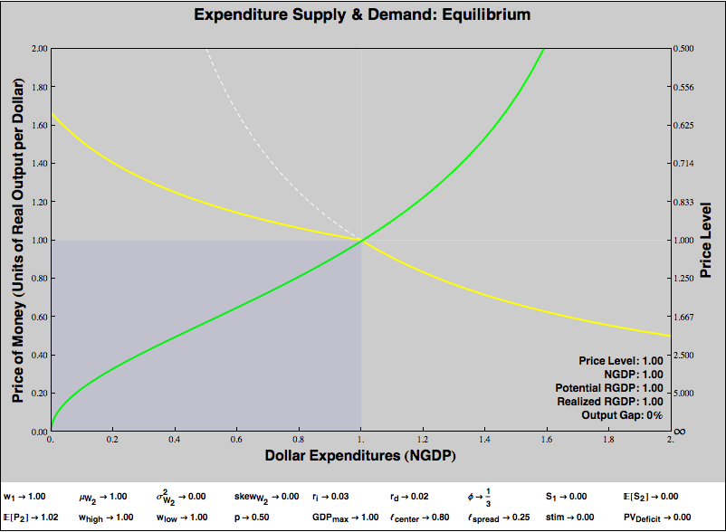
Below is a diagram of an economy in which demand shortfalls do not lead to output losses and money is neutral, because there are no price rigidities.
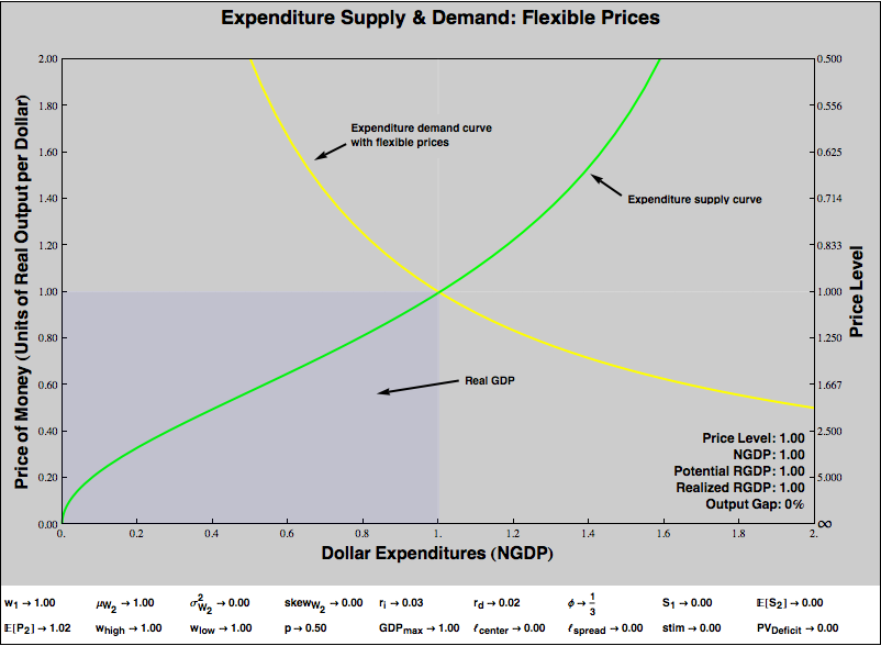
The downward-sloping yellow line is a demand curve, and the upward-sloping green line is a supply curve. Hopefully that seems familiar. However, we’re in a bit of a mirror universe, because we are graphing the supply and demand of expenditure. So the “expenditure suppliers”, represented by the green curve, are economic consumers. They supply dollars, for a “price”, which is some quantity of real goods and services. The “expenditure demanders” are economic producers. They demand dollars, but are only willing to offer so many goods and services for a buck. The equilibrium, the point where the two lines intersect, shows the price of a dollar, in real goods and services, that equalizes producers’ demand for money and consumers willingness to supply it.
For example, suppose that, at equilibrium, you can buy two widgets for a dollar. So the price of a widget is 50¢. But the price of a dollar is two widgets! Note the relationship — the dollar price of widgets is
(1 / PRICE_OF_DOLLARS_IN_WIDGETS)
This relationship is reflected on the axes if the graph. The left axis shows the price of money in real goods. If money is “expensive”, if you have to offer a lot of real stuff to get a dollar, that corresponds to a low price level, think deflation. Conversely, if money is “cheap” — if the equilibrium falls towards the bottom of the graph — then that means goods and services are expensive, think inflation. The right-hand axis shows the conventional price level, which rises as you travel vertically down the graph. As the price of money in real goods and services falls to 0, so you’d give up a dollar for next to nothing, the price level on the right-hand axis rises to infinity.
The X or quantity axis of the graph indicates how many dollars will be spent at the equilibrium. This has a very natural interpretation as nominal GDP. So, from the equilibrium point on the graph, we can read the price level (on the right axis) and the nominal GDP directly.
Real GDP is represented by the area of the bluish rectangle in the bottom left corner of the graph. To understand why, recall that real GDP is just
(NGDP / PRICE_LEVEL)
But the Y axis of the graph is
(1 / PRICE_LEVEL)
So the area of the bluish rectangle is
NGDP × (1 / PRICE_LEVEL) = (NGDP / PRICE_LEVEL) = RGDP
So what determines the shape of the expenditure supply and demand curves? Let’s start with demand. Suppose the economy produces at capacity and there are no “rigidities” to prevent the sale of all output. Producers will always accept however many dollars are on offer and sell the maximum achievable RGDP. Then
NGDP × (1 / PRICE_LEVEL) = MAX_RGDP
(1 / PRICE_LEVEL) = (MAX_RGDP / NGDP)
Since the inverse price level is our Y axis, and NGDP is our X axis, the function that describes our no-rigidity demand curve is just
Y = (MAX_RGDP / X)
which is the graph of a grade-school hyperbola. We’ll modify this shape a bit, when we start thinking about price rigidity. But let’s hold off on that.
What determines the shape of expenditure supply? That’s where all of the action is in terms of fiscal and monetary policy, and we’ll graph lots of funky shapes below. But fundamentally, the answer to this question is easy. Imagine a world of consumers, each of whom must decide how much to spend now and how much to save for the future. Suppose we can characterize consumers’ “intertemporal preferences” with a utility function. Then we can compute how much each consumer will spend. Naturally, that utility function will take into account the current price level, among other parameters. If we hold other parameters constant, we can compute how expenditure varies with the current level of prices. We add up all consumers’s expnditures and plot them on the X axis, against (1 / PRICE_LEVEL) on the Y axis. That gives us our expenditure supply curve.
Immaculate Deflation
In the graph above, everything has been normalized to one. The graph shows one unit of real goods “buying” one dollar of expenditures, for a price level of one. Suppose that consumers become more reluctant to spend money, that is, they perceive the marginal opportunity cost of parting with money as increasing. The result would be an “immaculate deflation”, in that expenditure would fall, but so would the price level, so that the reduced expenditure would still purchase all the economy’s real product, and RGDP would not fall at all. Here’s the graph:
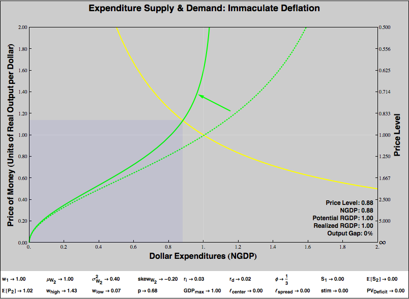
Note expenditures have fallen, but the quantity of goods offered for each dollar has risen. Real GDP — the area of the bluish rectangle — has not changed.
Price Rigidity
In the real world, when nominal expenditures fall, the quantity of goods offered for a dollar doesn’t rise enough to compensate. The quantity of goods purchased actually decreases. Let’s graph that:
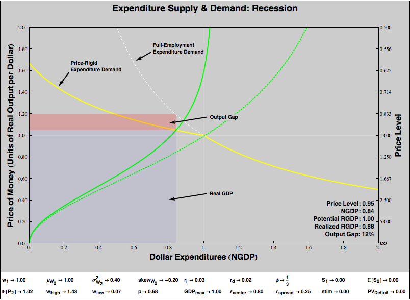
The expenditure supply curve is identical to that in the previous graph. However, the shape of the expenditure demand curve has changed. There is now a “kink”, that begins (as I’ve drawn it) just under the original equilibrium expenditure of one. Our steepened expenditure supply hits the kinked region, forcing that the quantity of goods offered for a dollar to be lower — or the price level to be higher — than in the previous graph, with its unkinked, flexible-price expenditure demand curve. This means that, given the reduced level of expenditure (caused, as before, by the steepening of the expenditure supply curve), the quantity of goods consumers purchase is less than the economy’s capacity. We observe a fall in real GDP and a recession.
As before, the area of the bluish rectangle represents Real GDP. The dotted white line shows the flexible-price expenditure demand curve, while the yellow line is the expenditure demand curve that actually obtains, with its kink and price rigidity. The reddish rectangle represents the output gap: the area that should have formed part of GDP, but does not because of the price rigidity.
In this example, the price level has from 1 to 0.96 (a 4% deflation), and real GDP has fallen by 10%. Note that in the previous example, with the same steepened expenditure supply curve but flexible prices, the price level fell even farther (to 0.88, a 12% deflation), but RGDP was unaffected. There’s an important bit of intuition here. We often imagine that deflation causes recessions, and indeed in our graph, we can see that deflation is associated with recessions. We would only see an output gap when the equilibrium fell before the kink in the curve, which is always a price level lower than our original price level. But under flexible pricing, the deflation would have been more severe, without harming RGDP. It is not too much deflation that creates the output gap, but too little deflation given the fall in expenditures! Tepid deflation is a marker of recessions, but it is the decline in nominal expenditure, in NGDP, that drives the show.
If you are wondering where the shape of the sticky-price expenditure demand curve comes from, see my earlier post on sticky prices. Basically, to generate the expenditure demand curve with price rigidity, I assume that industry leverage is uniformly distributed over some range, that firms in industries set minimum prices based in their degree of leverage, and that firms’ capacity is constrained in the short term. If you don’t buy that story, but agree that prices are sticky downward but not so sticky upward, then you can take the shape as an arbitrary qualitative depiction of that.
The Expenditure Supply Curve
Expenditure supply is where the action is in making sense of Keynesian and monetarist interventions. The nice thing about this framework is one can posit any intertemporal utility function you like for agents in your economy and then compute the shape of the expenditure supply curve as you vary parameters.
For the purpose of this exercise, I’ll adopt an unrealistic but illustrative utility function presumed to be shared by all consumers. Consumers will face a two period, rather than infinite horizon optimization problem. Their behavior will be based upon a number of factors, all of which are treated as exogenous parameters:
- An interest rate ri which determines the Period 2 value of money not spent in Period 1.
- An current wage w1, in nominal dollars.
- An expected future wage μw2, in nominal dollars.
- Variance of the distribution of future wages, σw22
- Skewness of the distribution of future wages, skeww2
- A current price level P1
- An expected future price level E[P2]. (Oddly, the current price level is what we are trying do determine. The expected future price level is known, and helps to pin the present price level.)
- A current taxes-and-transfers surplus S1.
- An expected future taxes-and-transfers surplus E[S2].
- A discount rate rd, which is the rate at which consumers discount future utility.
A “real” model wouldn’t treat all these parameters as free. For example, perhaps the expected price level is dependent upon current interest rates, or fiscal policy. My goal here isn’t to present a falsifiable model of consumer behavior, but to illustrate what proponents of various interventions are claiming, and explore under what circumstances they would or wouldn’t work. We will find, for example, that, running a Period 1 taxes-and-transfers deficit while holding interest rates constant increases Period 1 expenditures. However, this effect will be mostly undone if the Period 1 deficit must be balanced by a Period 2 surplus. We don’t wish to take a position here in the “Ricardian equivalence” debate. Allowing the two deficit parameters to vary freely, rather than enforcing some hypothesized relationship, permits us to illustrate the claims of partisans on both sides.
The utility function I’m using to compute the expenditure supply function is shown below.
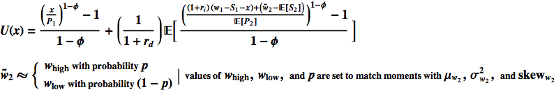
Our variable x represents nominal dollar expenditures.
There are a bunch of things about this utility function that are crappy, but I think it’s good enough to show how changes in parameters might affect a expenditure supply curve, and offer some intuition about how various interventions might work.
Although I’m using just one utility function here, a nice thing about this framework is that it need not rely on a representative agent. What we will derive, after all, is a Marshallian supply curve. We can define populations of agents with different parameters or preferences and combine the supply curves by “horizontal addition”.
Visualizing Changes in Expenditure Supply
Let’s start with a graph of an economy characterized by price rigidity, but which is currently at “full employment equilibrium”. (The scare quotes are because I am not explicitly modeling labor, so by full employment I just mean that the economy is producing at capacity.)
Now, suppose that for whatever reason, uncertainty surrounding future wages increases:
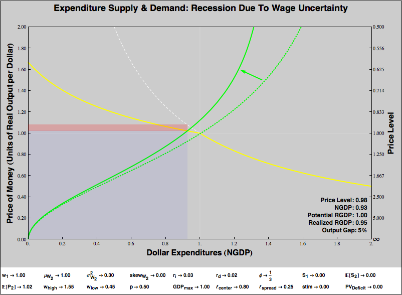
The expenditure supply curve steepens. Consumers become more reluctant to part with dollars, as they have been made worse off in the future and prefer to save. Unfortunately, after this steepening, the expenditure supply curve now intersects with the sticky-prices region of the expenditure demand curve. The resulting equilibrium is recessionary; the economy experiences a 5% output gap.
What kind of interventions might we try to fix this? Conventionally, our first resort is to discourage financial saving and promote current expenditures by reducing interest rates:
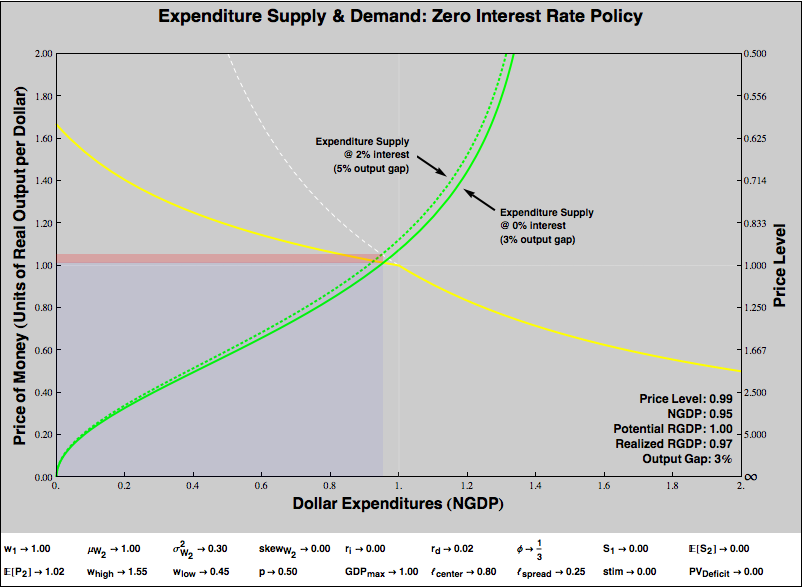
Dropping interest rates to zero helps, but it turns out to be insufficient, a 3% output gap remains. We have entered the liquidity trap, if you believe in such a thing.
But we are certainly not out of potential of interventions. Suppose we believe that the central bank is very, very good at setting expectations. Okay, if it were really great at that, it could just reverse the shock to consumers’ expectations of wage uncertainty and we’d never leave our initial equilibrium. But suppose the central bank can’t do that, but it can manage expectations of the price level. Then…
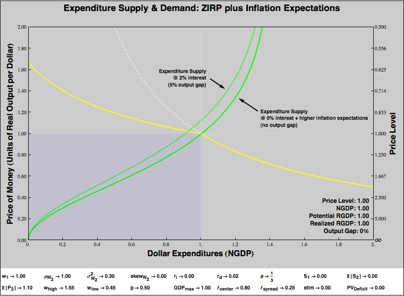
That worked! Yay monetary policy, still potent at the zero bound! But, we should be careful. We’ve assumed the central bank could set price level expectations. That’s much less sure than assuming it can set interest rates. Plus, perhaps engineering an uptick in inflation expectations is hazardous. Perhaps the central bank cannot set expectations precisely, so that there is a hazard of overshooting and generating inflation rather than just restoring equilibrium. Perhaps there is value to keeping inflation expectations “anchored”, and the change in expectations required to restore equilibrium would upset that anchoring. So, it’s worth considering alternatives.
Let’s go back to our original disequilibrium, and let the MMT-ers have their way. Suppose that to counter the 5% output gap, the government reduced taxes and/or increased transfers, to run a deficit. Could that work? Absolutely.
However, there’s a catch. My two period setup is pretty Ricardian. Encouraging private spending through a taxes and transfers deficit in Period 1 only works if that deficit is not repaid by running a surplus in Period 2.
However, in the real world, deficits needn’t be repaid via prompt surpluses, and economies (measured in nominal dollars) often grow faster than the interest rate paid on public debt. In this case, debt effectively repays itself over time, without ever requiring surpluses. The core new debate over MMT as well as a very old debate over “Ricardian equivalence” turn on the degree to which people have (or by tax policy can be made to have) a special willingness to hold currency and government securities even when doing so implies an opportunity cost relative to a hypothetical asset that matches the economy’s growth rate. I think the case is very strong that, under many circumstances, people are willing to bear that cost, not least because a hypothetical asset that earns the economy’s growth rate with little risk does not exist, and most people are more concerned with managing risk than with maximizing return.
(Note: If you think transfers that will never be paid for in taxes must increase the expected future price level, then in the immediate term, all that does is to reduce the scale of the program necessary to eliminate the output gap! An increase future price level expectations, like the unfinanced transfer itself, renders the expenditure supply curve shallower, helping carry our equilibrium out of the recession region. Of course, we are observing a one period snapshot of the economy, and there may be long-term bad consequences to “unanchoring” the price level. That’s beyond the scope of our little visualization, but that doesn’t mean we shouldn’t worry about it.)
My little experiment is not so friendly to a taxes-and-transfers-based “hard Keynesianism“, which prescribes prompt surpluses to offset cyclical deficits. In my toy model, a reduction of expected future income is very much like a reduction of present income, as agents can borrow and save at “the” interest rate. But this is not realistic: real humans pay more to save than to borrow, and may face outright credit rationing.
I give lip service to uncertainty by calling the future surplus “expected”, but I don’t actually model it as uncertain, as wages are the only random variable in my toy utility function. If I had, the cost of future surpluses to consumers would be even greater, and it would make “hard Keynesianism” look even worse. So implemented in terms of taxes and transfers, ignoring the wedge between saving and borrowing costs, and holding wealth distribution constant, it’s hard to see how one could ease a recession by running deficits which are expected to be balanced by prompt surpluses. Of course, these assumptions needn’t hold. We do not have to restrict ourselves to taxes and transfers, but can have government deficit-spend on real goods and services directly. Savers do, in fact, face liquidity and borrowing constraints that “hard Keynesianism” can overcome by effectively using the government’s balance sheet to borrow on behalf of consumers. And when we tax-and-transfer, we can also redistribute.
I yet haven’t tried to model consumers facing borrowing constraints. But I have played with variations in which government spends, rather than transfers its deficit, and with redistribution. So let’s look at those.
Stimulus Via Direct Government Expenditure
The economy’s true “expenditure supply” includes the inclination of government to directly purchase goods and services. Thus far we’ve ignored that. If we hold government’s propensity to spend invariant to the parameters of our toy model, ignoring government purchases doesn’t much hurt our analysis. But is that a realistic assumption?
It would be hard to model how government’s inclination to spend varies, and upon what parameters that variation depends. However, governments do sometimes respond to recessions by adopting stimulus programs, which in rough approximation we can model very easily.
Here’s how we’ll do it. We’ll imagine that the government first chooses the quantity of dollars it will spend on real goods and services, and then chooses what it will purchase. That sounds unobjectionable, but it’s really very sneaky, because it means that stimulus spending is not a function of the quantity of real goods and services offered for the money. So the expenditure supply curve due to stimulus is vertical. Including expenditure due to government stimulus simply shifts the expenditure supply curve to the right by the quantity of nominal dollars appropriated!
Let’s see, in the simplest case, how a stimulus program that is not expected to be paid for from an increase in taxes can combat a recession. The dotted green represents the expenditure supply curve in our 5% output gap recession, and the solid green line illustrates the intervention.
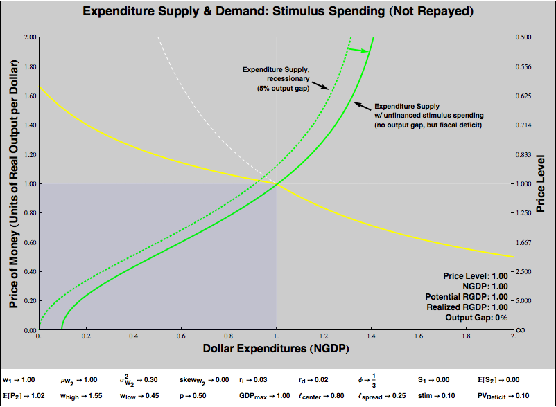
Note that the expenditure supply curve in this graph is different from all of our previous graphs. For ordinary consumers, the quantity of expenditure supplied always goes to zero as the price of a dollar in terms of goods and services falls to zero. The curve bottoms out at the origin of the graph. To put things in more familiar terms, if the price level today is infinite — you get literally nothing for a dollar spent — and the price level tomorrow is expected to be finite, you’d spend precisely nothing today. With stimulus via direct spending, the government commits to current-period expenditure regardless of the price level. The expenditure supply curve now bottoms out to the right of the origin.
Unlike a taxes-and-transfers deficit, stimulus via direct spending “works” under our toy model even if it is paid for via a fiscal surplus. It doesn’t matter, under our model, whether the spending is paid for out of current period taxation or future taxation. That is, our model suggests that it might be possible for a government to balance its budget in the teeth of a recession and still stimulate its way out of the recession!
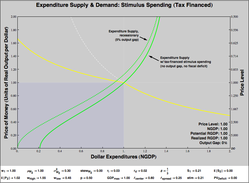
There is a hitch, of course. Our balanced budget is stimulative if and only if spending is increased and balance is accomplished by increasing current taxes. Cutting spending to balance the budget would be contractionary under our framework, while increasing taxes to fund spending is expansionary.
The intuition is pretty straightforward: Consumers divide current wealth between spending and saving. If consumer saving decisions compose to insufficient current spending to avoid recession, the government can preempt those choices by taxing current wealth and spending the entirety of the proceeds.
A few issues and caveats —
- Compare the graph above to the previous graph, where the stimulus spending is not funded by taxes. The X intercepts show how large the government’s spending program must be to eliminate the output gap. Unsurprisingly, government must commit to a great deal more spending to render a funded stimulus effective than it would need to for an unfunded stimulus.
- If the spending program were funded by future period taxes rather than current period taxes, the graph would look nearly identical, given the near-perfect substitutability of present and future money in our model. However, as we discussed above, in the real world, consumers find it expensive or impossible to borrow from the future in recessions, so transferring wealth to current consumers and taxing in the near future to pay for it may be directly expansionary. If that is so, then the scale of government spending required to cover the output gap would be smaller if the spending is paid for out of future taxes rather than out of present taxes.
- If a government commits to large nominal expenditures irrespective of what is to be purchased, indiscriminate spending decisions might degrade the quality and value of current output. If so, effect of the increase on current expenditures might be undone, partially or completely or worse than completely, by a supply-side losses. See “supply and technology shocks” below for an example.
Distributional Effects
Part of my motivation in developing this framework was to come up with a way of conveniently analyzing distributional effects. We can compute different expenditure supply curves for subpopulations of different wealth levels, and “horizontally add” those curves to get the economy-wide expenditure supply. I thought I would easily be able to define some very rough distribution parameter, and show how redistribution affects expenditure supply.
I began with a very strong prior: I believed, and still believe, that the poor are much more likely to spend out of current income than the rich, so that redistribution from rich to poor would increase current expenditures (that is, render the slope of the expenditure supply curve more shallow). To get a quick and dirty take on distribution, I compared two economies, one in which all the wealth was held by a single individual, and a second in which the wealth was equally distributed among many individuals. I expected a shallower curve in the second case.
But that is not what I found, under the utility function above. In fact, it is easy to show that, holding total real wealth (both current and expected future) constant, the expenditure supply curves are identical if the economy contains just one spender (while everyone else starves) or a perfectly equal distribution of wealth. So have I revised my priors?
No, not at all. Instead, I’ve understood deficiencies in my utility function, deficiencies that I think are shared with most utility functions used to build macro models. Why is expenditure supply constant, regardless of distribution? It’s pretty simple really. Under the terms of the model, agents are perfectly forward-looking and all wealth must be spent eventually. Intuitively, we think poor people will spend money today if we put it in their hands because the absolute cost of not spending — going hungry, for example — is large. But, given the structure of my and most macro models, agents don’t evaluate current expenditure against absolute gains in present utility, but against opportunity costs in future utility. If an agent is poor, sure, not eating today has a large cost. But eating today exacts a similarly large cost from the still-poor-me of tomorrow. A rich agent gains little by eating a bit more today, but her cost in future consumption for that benefit is similarly low. Under my utility function, as long as the two agents discount future utility identically, they will make precisely the same tradeoff between expenditures today and expenditures tomorrow. So a poor person, despite starvation, will be just as disinclined to spend current wealth as a rich person. The poor person will balance starvation tomorrow against hunger today, and save some fraction of her wealth. The rich person will balance the pleasures of a bon bon tomorrow against a cookie today, and save precisely the same fraction.
I think this is entirely unrealistic, but what’s interesting is to articulate why. Let’s think about it. In my model, all agents live for precisely two periods, no matter how much or how little they consume. In the real world, insufficient consumption today implies death and zero consumption in the future, regardless of how much a person might have saved. So a realistic model needs some concept of subsistence, such that as present consumption falls and the probability of death increases, the value of future savings is increasingly discounted. More generally and less drastically, future wages in my model are stochastic, but independent of present consumption. But that makes no sense. My ability to earn future wages depends upon my current expenditures. My distribution of future wages is dramatically different if I have a home, decent clothing, a telephone, or an education, than if I do not have these things. Ultimately, I need to add to my consumers’ utility function some notion of investment expenditure that impacts future wealth, rather than restricting the choices to pure consumption and financial savings for interest. And there should not be a single, economy-wide investment return, but each individual’s returns should (usually) be diminishing in wealth. My first dollar of expenditure buys me the ability to survive into tomorrow and enjoy potential future wages; its return is very high. Direct investment of my millionth current dollar might buy me an additional nice suit or make some marginal contribution to a business, but its effect on my future wealth is likely to be small. If I include this sort of direct investment in my model, I think I’d generate the expected relationship between poverty and a bias towards current expenditure. But that’s an exercise I’ve not yet done.
Technology and Real Supply Shocks
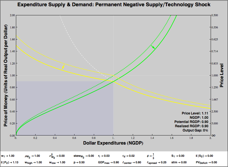
The supply side of our economy is graphical represented by the yellow expenditure demand curve. That curve is based on a hyperbola, whose numerator is the capacity of the economy in units of real output. A negative real supply or technology shock yields a recession, without any change in consumers’ willingness to spend:
Note that the output gap is 5%, just like demand-shock recession we’ve illustrated in previous graphs. However, this recession is actually much worse. The real output of our economy has fallen by 13%, not by 5%. The negative supply shock eliminated almost 9% from our potential output. Plus, even though the expenditure supply curve has not changed at all, the shift in the expenditure demand curve pushed the equilibrium onto that curve’s rigid price region, generating an output gap of 5% of our diminished potential output (about 4% of our original output) in addition to the loss of real capacity. In response to a negative supply shock, increasing consumers’ willingness to spend can eliminate the loss of output due to price rigidity, but cannot affect the loss of real capacity:
It’s worth commenting on how the shape of the expenditure demand curve as it shifts in response to a supply shock. By hypothesis, the “kink” in the curve is a function of nominal indebtedness. A firm that requires a dollar of revenue to service its debts doesn’t reduce the price of its total output below a dollar, even if a technology shock diminishes the quantity or quality of that output. So the kink stays where it began, at nominal expenditure of 1.
Yet consumers’ willingness to spend is a depends on the value of real output provided. Holding constant expectations about the future, consumers are less willing to provide that dollar of current expenditure for less or worse stuff. So despite a higher current price level — which you might think would ease the burden of servicing on nominal debt — the diminishment of nominal expenditure occasioned by transiently higher prices (the left-shift of the equilibrium) means that firms have a significantly harder time servicing their debts.
Note that, perhaps counterintuitively, our output gap arises because consumers are optimistic that the real supply shock is temporary. If consumers expect the supply shock were permanent, and therefore that the future price level would rise along with the present price level, a demand effect offsets the supply effect, and the output gap disappears. Consumers become more willing to supply expenditures now because they no longer expect tomorrow’s money to be more valuable than today’s. (The shift in the yellow expenditure demand curve is the real supply shock. The shift in the green expenditure supply curve shows the increase in current spending due to expectations of future high prices.)
“Stagflation” comes from any sort of negative real supply or technology shock, but is magnified when consumers believe the shock to be temporary!
This is an important difference between demand and real supply side shocks. If consumers’ inflation expectations are “adaptive”, that is, if we learn from experience to predict the future, then for supply shock, changes in expectations help stabilize the current price level and eliminate any output gap. For a demand shock, adaptive expectations about prices are destabilizing. If a demand-driven deflation means we expect future deflation, that diminishes our willingness to spend, which renders our current output gap and deflation even worse. Supply shocks self-heal, demand shocks self-destruct. (Remember, “supply shocks” are shifts in the the expenditure demand curve of our framework; “demand shocks” are shifts in expenditure supply!)
Of course, even if consumers do believe a real shock to be temporary, the output gap can be eliminated by expansionary monetary or fiscal policy. However, no amount of monetary or fiscal policy can undo the real shock. If potential real GDP has fallen by 10%, encouraging people to spend can eliminate the output gap due to price rigidity, but cannot (in a static sense, at least) bring back the lost potential output.
Until the last graph, we’ve considered changes ceteris paribus, adjusting one or two parameters and imagining that all the rest can be held constant. But of course, most of the controversy surrounding proposed policy interventions is about the way in which various changes are interrelated. So, for example, earlier we showed a graph in which stimulus spending eliminated the output gap from a demand shock. However, those who oppose stimulus often argue that poorly targeted government spending will reduce the quality of real output delivered by the economy. Thus, a demand-side remedies will provoke a reduction of real supply. Let’s illustrate that claim:
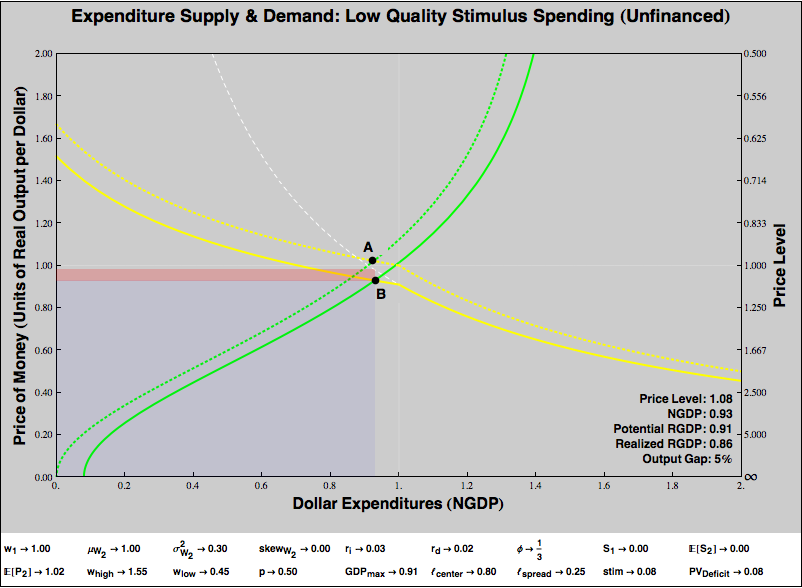
Point A on the graph represents a demand-driven recession, the same recession we graphed in Figure 5. If we left it alone, the economy would face a 5% output gap. That sucks, so we try fiscal stimulus, exactly as we did in Figure 9. Unfortunately, although we successfully shift the expenditure supply curve, poorly targeted government spending leads to suboptimal real production. The expenditure demand curve shifts downward. We end up in a different recession, a worse recession in this example, at Point B.
So what does our analysis say? If we use stimulus spending to counter a recession, will it lead us towards the happy outcome diagrammed in Figure 5 or the terrible outcome diagrammed above? I don’t know. As we said at the outset, our toy model is designed to illustrate possibilities, not to choose among them. But he have learned something about how to consider the question. If government spending is of sufficiently high quality that it doesn’t much reduce the value of aggregate output, then it likely can counter demand-shock recessions. If government spending is of such poor quality that the value of aggregate output is impaired by its psychotic purchaser, than stimulus spending may prove badly counterproductive. People’s views on the quality of government expenditures tend to correlate with tiresome political affiliations. My own view is that we have free will, collectively as well as individually, that governments sometimes do deploy resources wisely, but sometimes they make choices that are awful and corrupt. Our work is not to estimate the odds, but to shape the context in which government acts so that it is likely to act well.
If you think this story argue for monetary expansion as opposed to fiscal stimulus, think again. We can tell almost exactly the same story. Expansionary monetary policy, like government spending, increases our aggregate propensity to spend. But who says it has no effect on the production side of the economy? My own view, with the Austrians and other cranks, is that stimulating demand via low interest rates does cripple real supply over time, in part by favoring producers of durable goods, but more insidiously by altering the incentives of holders of financial assets, who diversify to capture monetary policy subsidies rather than discriminate between worthy and unworthy enterprises. I would rather take my chances with more transparent (if transparently corrupt) fiscal policy than with status quo monetary policy.
But that’s just me. The framework we’ve set up can illustrate happy and tragic stories, for both monetary and fiscal interventions. Further, if we come up with models that specify relationships between the parameters, or between the demand side and the production side of the economy, we can illustrate those models with the same sort of graphs we’ve shown here.
We’ve been working with a discrete, two period toy model. However, that’s limiting. For example, if poor government spending harms the supply side of the economy, the effect may not be simultaneous. We’ve crammed several non-instantaneous effects into “Period 1”. But we can draw graphs like this as “snapshots” of models that evolve over time. We can even combine graphs into annoying little movies to watch the economy evolve under various scenarios.
This has been a long exercise, and I’m grateful to readers who’ve made it this far. I’ve learned a lot from playing around with these graphs, but I’ve no idea whether doing so will help others. I hope so!
If you haven’t yet, do try playing around with the interactive graphs here. (You’ll need to install the Mathematica plug-in.)
- 28-May-2011, 8:00 a.m. EDT: Many thanks to JKH, fixed the explanation of Figure 1, which confusingly referred to the Y axis as the X axis.
[…] Visualizing Keynesian & Monetarist recessions Steve Waldman. Wonks will have great fun with this one… […]
May 27th, 2011 at 3:24 am PDT
link
[…] den makroøkonomisk debatten om stimulanser, rentesetting, Keynes og monetarisme har Steve Waldman skrevet en veldig god bloggpost hvor han tegner og forklarer. Noen ligninger og modeller er med, men intuisjonen får man med seg […]
May 27th, 2011 at 5:04 am PDT
link
Great work! Just one quibble.
You’re absolutely right in asserting the commonalities between monetarists and New Keynesians – almost all the differences between them are ideological. But I think you’re a little unfair in lumping the Post-Keynesians with them. The fundamental difference between Post-Keynesians (Minsky, GLS Shackle, Paul Davidson) and the rest is that they don’t rely on sticky prices/wages. And working from Keynes’ 1937 QJE article and Chapter 12 of the General Theory, they emphasise the impact of radical uncertainty and financial markets on investment expenditure. There are a lot of things on which I disagree with the Post-Keynesians but just on the above (especially Minsky’s thesis) I tend to agree.
May 27th, 2011 at 7:27 am PDT
link
“Perhaps the central bank cannot set [inflation] expectations precisely, so that there is a hazard of overshooting and generating inflation ”
Are you saying that expectations-setting is a sham? That they set expectations of higher inflation to spur growth, while intending to deliver a lower level of inflation once the growth has arrived? If so, it’s no wonder that credibility is an issue…
May 27th, 2011 at 11:29 am PDT
link
Isn’t your revelation about the distributional effects in the model just a restatement of marginal-utility theory? If you have only a few dollars, another dollar has higher utility than if you have a lot of dollars. Being able to put your two kids through university delivers more utility than buying a second or third Lamborghini.
So shouldn’t the utility function be adjusted for income, or even better, wealth? (Because we spend out of wealth, not income.) Could be simple, like:
Marginal utility of an additional dollar = 10-log(wealth)
This assumes that if you have 10 billion dollars, an additional dollar is essentially valueless to you. Here’s what it looks like as you move down the wealth ladder:
Wealth Marg. Util.
10,000,000,000 0.0
5,000,000,000 0.3
2,500,000,000 0.6
1,250,000,000 0.9
625,000,000 1.2
312,500,000 1.5
156,250,000 1.8
78,125,000 2.1
39,062,500 2.4
19,531,250 2.7
9,765,625 3.0
4,882,813 3.3
2,441,406 3.6
1,220,703 3.9
610,352 4.2
305,176 4.5
152,588 4.8
76,294 5.1
38,147 5.4
19,073 5.7
9,537 6.0
4,768 6.3
2,384 6.6
1,192 6.9
596 7.2
298 7.5
149 7.8
75 8.1
37 8.4
19 8.7
9 9.0
5 9.3
If you’re broke, a dollar is worth 31 time as much as if you have five billion dollars. I’d make it far steeper, especially at the bottom, perhaps shape it differently than a log curve, but it shows that you can fashion a intuitively reasonable wealth-based utility function fairly easily. Not sure how it would wire into your Mathematica model.
May 27th, 2011 at 12:14 pm PDT
link
Very nice discussion, but it misses what that I think is Keynes’ most
important lesson.
You get so close here:
“… future wages in my model are stochastic, but independent of
present consumption. But that makes no sense.”
but the next sentence disappoints:
“My ability to earn future wages depends upon my current
expenditures.”
This statement is certainly true; but current expenditures impact
future wages in another, critical way: if you spend money, someone
else has it, which means they can spend it in the next period, perhaps
on your services. Of course, if one is a small individual agent in a
large economy, one recovers only a tiny fraction of one’s expenditures
by this mechanism, so micro-economists rightly neglect it. The macro
economy taken as a whole, however, recovers *all* expenditures by this
mechanism, so it has a huge, multiplicative impact on total output.
That’s why they call it the multiplier.
During recessions, the output gap is an instance of the tragedy of the
commons. The effect of my expenditure on my future wages is
negligible (except by the self-investment means discussed in the
essay), but the effect of aggregate expenditure on aggregate future
wages is huge. When the economy is in full employment this only
produces inflation, but during a demand-recession getting everyone to
increase spending produces real wealth because it closes the output
gap first.
May 27th, 2011 at 3:19 pm PDT
link
Nothing against math, but post-Keynesian MMT is the way to go. Trying to accommodate all the schools of thought makes it more complicated than it needs to be, unless you are trying to reason with people steeped in the misguided schools of thought. Nothing wrong with that, but I would encourage those who just want the important stuff to stick to MMT…
May 27th, 2011 at 10:36 pm PDT
link
Very creative and cool.
(I’m guessing quasi-monetarists might like this.)
Tiny typo time:
Shortly following figure 1, should be:
“But the Y axis of the graph is
(1 / PRICE_LEVEL)”
Question re the following:
“There’s an important bit of intuition here. We often imagine that deflation causes recessions, and indeed in our graph, we can see that deflation is associated with recessions. We would only see an output gap when the equilibrium fell before the kink in the curve, which is always a price level lower than our original price level. But under flexible pricing, the deflation would have been more severe, without harming RGDP. It is not too much deflation that creates the output gap, but too little deflation given the fall in expenditures! Tepid deflation is a marker of recessions, but it is the decline in nominal expenditure, in NGDP, that drives the show.”
If leveraged firms defend the “Waldman kink” by resisting further price decreases along that curve, but at the same time there is a GDP opportunity cost due to insufficient deflation, doesn’t that mean that the same firms have foregone revenue as a result? And doesn’t that mean they’ve missed out on generating higher income to capital and labour? And doesn’t that mean that they’ve missed out on higher return on equity and a lower probability of bankruptcy by deflating further?
How do you reconcile their original strategy (i.e. probability distribution for bankruptcy; chosen line (kink) of defense) with this? Is there any contradiction? (I’m probably missing something simple here.)
May 28th, 2011 at 6:04 am PDT
link
Ashwin — So, I don’t want to get too bogged down in the sort of ideological squabbles I’m trying to circumvent. But I think that the post-Keynesians, especially the Minsky acolytes (among whom I’m proud to count myself, to a degree), do in fact rely upon sticky prices, although they don’t use those words. The core of Minsky’s model of the economy is that “profits equal investment”, that is, the price structure of the economy must be set such that there is a sufficient mark-up over the direct labor costs of production to cover all of the secondary and indirect costs, including especially the cost of producing capital goods. In an economy in which investment goods are funded over time via financial commitments, the economy’s mark-up must produce sufficient profit to “validate” (Minsky’s delightful insightful term) capital commitments previously undertaken. Failure of this condition is how “it” would happen again, meaning a depressionary debt-deflation dynamic.
Minsky does not (as far as I know) posit a microeconomic story about how firms might resist pricing that would preclude validation of their commitments. (That’s what I’m trying to do with my leverage and sticky prices schtick.) But it’s clear that his account is incompatible with flexible prices, just arithmetically. This is easy to explain if you’ve followed my graphical reasoning. In Minsky’s world, full employment real GDP, at a point in time, under a given technology, sociology, and price level, is essentially fixed. (Minsky models it as a multiple of direct-production wages, which fraction of total wages would be technologically and sociologically determined, and which under full employment are fixed.) Above the price level necessary to pay diret wages and validate firm capital structures — above the “kink” in my diagrams — nothing bad happens. But, should total income fall below the “kink”, Minsky predicts that “it” happens again, implying that somehow, real GDP collapses. If real GDP — the area of a rectangle at the bottom left corner of my diagrams — collapses below a certain price level, arithmetically that implies an expenditure demand curve that falls somewhere below the hyperbola. It might not have the shape I describe or be perceived at a microlevel as sticky prices, but an implication of Minsky’s view is that a fall in expenditures that is not resisted leads to pricing that is above what would obtain under full production and flexible prices. You might dislike describing this as “sticky prices”, preferring to call it a collapse of real production concomitant with higher prices due to scarcity. But we are just giving different names to the same phenomenon. An implication of any sticky price account of depressions is that there is a glut of capacity at the sticky price level that is resolved by unemployment (of resources in general, but especially labor). We can tell a story that goes “sticky high prices” -> “temporary overcapacity” -> “financial collapse of many firms + underemployment”, or we can tell a story that goes “financial collapse of many firms + underemployment” -> “high prices due to scarcity” , but we end up in the same place. At a macro level, the economy cannot allow prices to adjust downward smoothly, in a manner consistent with maintaining full production. Prices, while they may fall in absolute terms, cannot adjust downward sufficiently to accommodate full production. (Note that by “high” prices, I mean high relative to flexible pricing. What we observe when “it” happens is deflation in absolute terms, but high prices relative to what would be consistent with both full-employment production and observed nominal income.)
Minsky, like any sticky price theorist, therefore suggests that nominal income must be stabilized above the “kink”, at levels that validate business structure commitments, in order to prevent “it” from happening. He points out that in modern economies, that’s exactly what central banks and governments do (first via lender-of-last-resort operations to prevent financial collapse, then via deficit spending to support nominal income). And he observes that this approach imparts an inflationary bias to the economy.
I don’t want to claim that there is no important difference between a vision of flexible prices that imply a collapse of real production and New-Keynesian-ish stories that suggest rigidity due to inherent but somewhat mysterious “menu costs” and such. But at a macro level, downward-sticky absolute pricing and a Minskian vision look very similar. And if we replace stories of menu costs or sequential price adjustment with a micro story about firms refusing to set prices below a solvency threshold, the sticky prices and Minskian stories come to look very much alike.
May 28th, 2011 at 8:14 am PDT
link
Steve R — So I’ve circumvented a lot of questions about setting inflation expectations (and important distinctions between price level and inflation expectations) by using a two period model. In a two period model, expectations of the next period price level and an expected inflation rate contain the same information. Had I used a longer model, I’d have to be careful. Agents might have an inflation expectation that is independent of isolated changes in the price level, so a central bank / fiscal authority could might have the freedom to adopt policies that cause a one-time jump in the price level without creating expectations of an increased inflation rate. Ultimately it is expectations about the sequence of price levels, not the inflation rate per se that determines expenditure, unless you want to make a case for including the inflation rate per se, rather than just the expected consumption value of expenditure in the utility function. But to say that inflation expectations may be distinct from isolated price level expectations is short-hand that says something (fairly loose) about the expected shape on the long-term series of price levels. If we say that a central bank commits to price-level targeting rather than inflation targeting (and if people believe that commitment), that implies a much stronger constraint on the shape of expected future price levels (any isolated “misses” will be corrected, so long-term prices are more predictable than under an inflation commitment).
May 28th, 2011 at 8:29 am PDT
link
Steve R @ 5 — So the utility function I’m using does imply declining marginal utility of expenditure. That’s already wired in. My “revelation” (and it was that) is that this alone is not sufficient to imply greater expenditures when you are poor. In absolute terms, sure, a poor person gets a lot more value from an additional dollar of expenditure than a rich person. But a poor person also faces much larger costs from an additional dollar of expenditure, in terms of consumption lost next-period. So, counterintuitively, a poor person is as unlikely to spend an additional dollar on a desperately needed meal as a rich person is to spend an additional dollar on a third scoop of ice cream. The poor person desperately needs a meal now but also desperately needs to save for her next meal. A rich person gains almost no benefit from the extra scoop of ice cream, but loses almost nothing in terms of the value of future consumption for indulging.
That the fraction of total wealth expenditure is invariant to total wealth does depend on my choice of utility function, but not in any way that redeems the intuition that the poor spend more than the rich because the absolute value of a unit of consumption is higher. [The fraction of expenditure would also be invariant under Log utility, which is a weird special case of the utility function I used. Playing around with CARA utility, whether rich or poor spend more present wealth depends on the relationship between the interest rate and the utility discount rate, among other things.]
You really do need to introduce extra features — features that are usually not introduced into macro models — to capture the intuition that if a poor person has $1 and a sandwich costs $1, she will spend her whole dollar today, while a person with $100 will spend a much smaller fraction of her wealth. Diminishing marginal utility just won’t take you there.
May 28th, 2011 at 9:47 am PDT
link
Alexey — We are talking across each other, I think. In the sentence you quote, I am discussing distribution: why would an individual agents future income depend on present expenditure? As you say, the macroeconomic effect on any individual of such expenditure is minimal. The aggregate effect on future income of increasing current expenditure may be large, but that doesn’t tell us anything about the distribution of wealth among individuals in future periods.
Putting aside distributional questions, we could sort of to model a Keynesian multiplier intuition by letting expected w2 be a function of expenditure rather than exogenously imposed. Our model becomes a “representative agent” model then, because doing that makes no sense for an individual, unless we assume that everybody gets the same w2 as a function of what everybody spent in period 1. But that would be fun to try. In terms of this model, adding a positive relationship between future wages on present expenditure would presumably reduce the slope of the expenditure supply curve (increasing the amount of expenditure for any price).
Note that under my framework, the only way that anything about future wages can impact present expenditure is through expectations. That’s not at all inconsistent with Keynes, who has people planning expenditures based on present knowledge, but those plans don’t always compose well. The multiplier effect is not something planned by individual consumers or firms, but describes the way in which plans either do or don’t work out in aggregate. Including an expectation that present expenditure increases future wages is an odd mix of Keynesian intuition and rational-ish expectations. Keynes doesn’t really expect individuals to consider the macro effect of their plans. The question of how future income expectations are actually formed, and under what circumstances that leads to present behavior consistent with those expectations being ratified, is an interesting one. Of course, if everybody expects awful future income, they might help ratify that by spending little today and causing a depression. More interesting is under what circumstances people have reasonably good expectations and their present behavior composes (perhaps with the help of government or a central bank) to make those good expectations transpire.
May 28th, 2011 at 10:11 am PDT
link
Detroit Dan — I guess a meta-case I’m trying to make is that we are drawing lines to sharply.
I read a lot of MMT papers now, and it bugs me how frequently authors explicitly speak to only one another, invoking the post-Keynesian tradition or speaking from the perspective of a “progressive economist”. That’s a strategy for staying marginal. If you think MMT has much to offer at the level of ideas (and I do), it’s probably counterproductive to require everybody to abandon their existing affiliations and join an explicitly progressive, post-Keynesian project. The ideas behind MMT can be translated into terms that “mainstream” and even “neoliberal economists” can make sense of, and can be used in pursuit of goals that even “Austrians” or “conservatives” might approve of. I hope to put things into terms that people of a variety of affiliations can make sense of, and point out how seemingly opposed camps might disagree less than they think. At some level this might be futile — people with different associations and sensibilities want to define themselves in opposition to one another, and intellectual differences are sometimes just an excuse for the fight.
But I hope that, to some degree, ideas do motivate people, and finding common ground for conversation might improve our understanding of one another’s perspectives and even create space for better policy.
May 28th, 2011 at 10:34 am PDT
link
JKH — Thanks a ton for finding that error! I’m really hoping that people try to make sense of these graphs. It doesn’t help if my explanations are incoherent.
Re the kink and foregone revenue:
Aggregate revenue, in the diagrams, is expenditure on the X axis. If you look at a recession (e.g. Figure 3, you’ll see it’s usually true that firms in aggregate would have higher revenue in expectation if they dropped to flexible prices.
Let’s consider a single, capacity constrained firm. (As we discussed ad nauseam in earlier comments the capacity constraint can be eliminated and replaced with a claims about the distribution of sales, e.g. that the variability of sales is limited. But capacity constraint is an easy way to form the intuition.) The firm requires nominal revenues of $0.95 in order to service its commitments and avoid bankruptcy. The firm will set a minimum price (but it can choose a minimum price of zero if it wishes, so we lose no generality.) The firm can produce 1 unit of goods.
Here’s a graph of a single leveraged firm. The horizontal line represents it’s minimum price (as 1/min_price, but you can read the minimum price off the right axis).
The firm sets a minimum price of $0.95. The intersection of its very kinked expenditure demand curve (representing the firm’s willingness to supply real goods) and the expenditure demand curve (representing demand for the firm’s products) shows the firm’s expected outcome. In expectation, the firm will sell only 0.86 units for a price of 0.94 units for $0.95, earning a total revenue of $0.89. In expectation, the firm is bankrupt.
But in expectation, the firm produces below capacity. The flexible price demand curve (the hyperbola including the curved part of the yellow line and the dotted white line), represents the firm’s capacity constraint. At the price of $0.95, if demand turned out to be more than expected, the firm could survive. If, at 95¢, the firm were to sell its full capacity, it would survive.
No consider a firm which prices its goods according to the flexible-price expenditure demand curve. That’d be the equilibrium where the green line meets the white dotted curve. Given the expected expenditure supply (consumer demand), it sets its price at $0.91. In expectation, the firm will sell its one full unit, and earn a total revenue of 91¢. 91¢ is more than 89¢, so in expectation, this is a better outcome.
Except that the firm is still bankrupt, equityholders still get nothing. Under the flexible price equilibrium, there might be a downside surprise to sales, but there will be no upside: the firm is expected to sell its full capacity. So, if the firm prices according to the flexible price equilibrium, it is bankrupt with certainty.
One way of understanding the capacity constraint is that it limits the area of the blue rectangle under the chosen price. The area of the rectangle can be no greater than one.The graphed firm, the one that set a minimum price of $0.95, can see that rectangle expand horizontally to 0.95, because its expected area is small. A firm that set its price according to the flexible price equilibrium’s expected outcome would include both the red and green rectangles, whose areas sum to 1. There is no room for rightward expansion along the revenue axis (X axis).
As long as equityholders control the firm (under our assumption that capacity is constrained and/or the width of the sales distribution does not much grow with falling prices), they will set the price no lower than $0.95, because at that price they have a shot of paying their debts. So the yellow expenditure demand curve will have the “dipper shape” shown. In expectation, the firm foregoes revenue by adopting this shape, but it preserves a lottery ticket to solvency. A firm could increase revenue in expectation by adopting a flexible price, but surrenders any chance of avoiding bankruptcy.
The expenditure demand curves drawn in the main body of the post are produced by “horizontally adding” dipper-shaped curves like the one shown, whose “kinks” are uniformly distributed around some average leverage value. This corresponds to a variety of industries, each of whose firms have very similar capital structures, in an economy with a given average leverage value.
(Some notes: I’ve treated revenue as synonymous with EBIT. Threshold sales — the location of the kink — would change, but little else, if we properly considered EBIT rather than revenue. Leverage conceptually includes operating as well as financial leverage, if the cost of failing to meet high fixed expenses is sufficiently disruptive to the value of the firm.)
May 28th, 2011 at 12:07 pm PDT
link
Thanks for the response, Steve. That makes good sense.
The way I see things is that MMT is correct on first principles, and the other perspectives aren’t. The issue of solvency versus debasement is one example of this, the endogenous nature of money is another, and the significance of horizontal and vertical transactions is a third. It’s hard to have a meaningful discussion when fundamentals aren’t acknowledged or discussed meaningfully.
In my experience, conventional New Keynesians refuse to discuss these fundamental ideas, but rather shift the discussion into details that just obscure things. Krugman and Quiggins come to mind. But you are different, and I appreciate that…
May 28th, 2011 at 12:48 pm PDT
link
Thanks for your explanations, Steve. As usual you’ve already incorporated much that I’m still flailing with. Also thanks for indulging tangents that don’t cut to the central point of the post (resolving different schools’ modeling approaches).
o As usual you’re right: the revelation is an “aha.” Without some wealth-indexed adjustment to current-versus-future spending predilections, ricardian equivalence (correct term?) means that marginal utility doesn’t affect propensity to spend now versus later at different wealth levels. Welfare economists hadn’t figured that out?
o You characterize Figure 5 as modeling “uncertainty surrounding future wages increases.” But isn’t it actually modeling low *expectations* for future wages? “they have been made [predictably?] worse off in the future.” Higher uncertainty would imply equal chances of higher or lower. Perhaps w[sub]2 models this in a way I don’t understand, with wage uncertainty causing lower wage expectations.
o I understand how incorporating investment as you suggest would model higher current expenditures by those with less wealth, and that may suffice in the model to roughly adjust for current versus future spending at different wealth levels.
But I wonder if accurate modeling wouldn’t require wealth-adjusted certainty and risk-aversion functions. (Maybe CARA and its cousins do that — as usual you’re way ahead of me.)
If we characterize the downside at the bottom end as suffering rather than starvation (or more generally failure to provide for future income hence consumption), and couple that with lower certainty among the less-wealthy, that would predict higher consumption expenditures, especially at the bottom end. “I know this will make me feel good/better right now, and I really don’t know what the future holds.”
o I’m not sure since you sort of reverse the supply and demand curves here — does this:
“different expenditure supply curves for subpopulations of different wealth levels, and “horizontally add” those curves to get the economy-wide expenditure supply.”
Run foul of the Sonnenschein–Mantel–Debreu theorem that Steve Keen makes so much of in Chapter Two of his book? (He also zeroes in on distribution as the crux issue: changes to price levels affect income distribution which affects demand curves which…)
Related: “deficiencies that I think are shared with most utility functions used to build macro models. ”
This (obviating the current/future spending effects of marginal utility via ricardian equivalence) appears to shoot a gaping hole at the waterline of most welfare economics models. Keen would certainly agree, though he states his reasons in different — though roughly equivalent? — terms. (He would also point to “static”/periodic modeling as the culprit, and he offers us a downloadable/executable dynamic simulation model as an alternative.) I’m assuming you wouldn’t go so far, but…?
May 28th, 2011 at 12:57 pm PDT
link
”
under flexible pricing, the deflation would have been more severe, without harming RGDP. It is not too much deflation that creates the output gap, but too little deflation
”
~~JKH~
The nutshell
But government rulers always do opposite to the remedy. They always try to prop up prices with clunker cash. They always try to extend the slow down just for the chance to buy in at the bottom of the Ponzi when things hit bottom 4 years later.
You can read their minds
!
May 28th, 2011 at 10:02 pm PDT
link
Thanks for that, Steve.
I utterly botched the relationship between nominal and real in my question.
This is a post worth investing time in – like learning a new language.
May 29th, 2011 at 12:06 am PDT
link
[…] Visualizing Keynesian & Monetarist recessions – via Interfluidity- So this will be an unusual post, more picture book than essay. Plus, it’s interactive! If you are willing to install the Mathematica plug-in, you can be the central banker / fiscal authority of your very own graphical economy! […]
May 29th, 2011 at 12:30 am PDT
link
I downloaded the plugin, played with it, and tried to read the posting. But it was too much for me to get through entirely. As JKH said, it’s like learning a new language; i.e. interesting but very time consuming.
The main point seems to be “the post-Keynesians, especially the Minsky acolytes (among whom I’m proud to count myself, to a degree), do in fact rely upon sticky prices, although they don’t use those words.” And you make an interesting case in that regard (in comment number 9, in particular).
However, MMT advocates claim that savings leakages also lead to output gaps and recessions. For example, if I buy government bonds rather than spending all of my income, that money is withdrawn from the economy. Isn’t that another difference between MMT and the other models? If so, could you adjust your model to take that into account?
May 29th, 2011 at 8:41 am PDT
link
Here’s a quote from MMT guru Bill Mitchell regarding savings leakages:
May 29th, 2011 at 5:42 pm PDT
link
I thank Steve Waldman for a stimulating and provocative artice.
I’ve been trying to understand the Expenditures Supply and Demand graphs. As noted, these graphs are mirror images of the usual supply and demand graphs. Along the top of the Expenditures graph could be entered an axis of Quantities (of goods and services) to go along with the Prices on the right hand side. (Am I correct that this Quantities axis is similar to the blue RGDP rectangle in the bottom of the left corner, and that a presumed blue rectangle in the upper right hand corner (prices times quantities) would be similar to the Expenditures axis at the bottom of the graph? If so, strange.)
I tried thinking of S&D graphs as generalizations of a single exchange, say a house sale. Suppose a house buyer is willing to pay up to $140k for a house, but no more. Because he owns and can supply dollars, he looks upon the dollar as the “numeraire”; he is willing to exchange one dollar for 1/140k (or more) of house. Similarly, suppose a seller putting a house on the market is willing to sell it for $130k, but no less. Because he owns and can supply the house, he looks upon the house as the “numeraire”; he is willing to exchange one house for $130k (or more). We normally think of money as the numeraire, as it is in regular S&D graphs, but in the expenditure S&D graphs, the goods are the numeraire.
If the prospective house buyer and seller reach an agreement and the house is sold, the selling price that actually occurs will fall somewhere in a field between the prices of $130k and $140k. (One could look at this field, among other things, as comparative advantage or arbitrage opportunities; economic fields occur whenever different parties place different valuations on items to be possibly exchanged)
Before the actual sale occurs, all prices in the field, between $130k and $140k inclusive, are merely potential (expected? hoped for?) prices. But then, how is the actual price determined? Where on the supply curve will it fall? Will it be the buyer’s maximum price of $140k, which the seller would be happiest with, or the seller’s minimum price of $130k, which the buyer would be happiest with, or something in between? The potential price that will be actualized depends upon the relative bargaining power of the seller and buyer. How desperate is the seller to sell or the buyer to buy? What other houses are on the market? How many other potential buyers are around.? How much money does the buyer have? Power–a concept that seems to be concealed in economics–enters into the determination of prices as well as most everything else.
In the graph “Expenditure Supply & Demand: Flexible Prices” the prices of money in terms of real output, the regular prices, and the potential, nominal and real GDP are all set at one. Presumably the sellers of money might have preferred lower prices, and the buyers of money higher prices. Thus the actual prices represent some kind of accommodation between the sellers and buyers.
In the graph “Expenditure Supply and Demand: Immaculate Deflation,” the shrinkage of expenditures by the money sellers, as pictured by the changed expenditure supply curve, pushes down the prices received by the goods sellers/money buyers; prices decline from 1.00 to .88. The goods sellers/money buyers lose clout; they produce as much as before (1.00), but their incomes decline from 1.00 to .88.
In the graph “Expenditure Supply and Demand: Recession,” the goods sellers/money buyers gain some of the clout that they lost earlier, as pictured by the changed expenditure demand curve; their prices rebound from .88 to .95 (?.95 on the graph, .96 in the text), but the goods (RDGP) available to the money sellers/goods buyers decline from 1.00 to .88.
It seems that shifts or changes in the shapes of supply and demand curves represent changes in the clout of sellers and buyers, of producers and consumers.
Some questions: Under what conditions do households, businesses, governments, and foreigners act as money sellers (expenditure suppliers)? Similarly, under what conditions do households, businesses, governments, and foreigners act as goods suppliers? And what about the financial institutions that “create” the money (“expendditures”)? What about debt? Do the financial institutions create any “goods”? If so, does their “production” belong in the top Quantities axis or the bottom Expenditures axis? Would “financial production” be considered Real production or Nominal production? If the later, should it be adjusted as nominal prices may be? Any answers or suggestions as to how to find answers to the above and similar questions, as well as any corrections or criticisms of the above analysis, would be appreciated. (allis 2@cox.net)
May 29th, 2011 at 7:24 pm PDT
link
Steve R —
Re: distribution — That something is a revelation to me doesn’t mean that it’s not been noticed by others. I’m sure this point has been made. But nevertheless, it remains the case that most “microfounded” macro models are built on frameworks that fail to reproduce obvious distributional effects. This might not be so consequential, since most macro models assiduously avoid considering distribution, allowing for some “representative agent” to stand happily in for everyone. But even those models might miss a lot by failing to take into consideration the path-dependency of consumption, or what you and I might call “investment” that takes some form other than letting mere non-consumption magically transform into undifferentiated capital.
Re: uncertainty: In both Figure 4 and Figure 5, the expected or average wages are 1. On the graphs you can read expected future wages directly; it is the parameter μw2. In Figure 4, agents expect to receive wages of 1 with perfect certainty. In Figure 5, agents expect to receive wages of either 0.45 or 1.55, each with probability 1/2. So, on average, agents expect to receive a dollar. But they still reduce current expenditures, and consider themselves worse off. The utility function I am using implies risk aversion. In fact, risk aversion is precisely a consequence of the declining marginal utility we were discussing before.
To see this suppose that my utility for $1 of certain income is exactly 100. Suppose instead of $1, I receive $1.50 of income. How much utility will that give me? Something more than 1. Let’s call it, arbitrarily but for the sake of discussion, 140. Now suppose I receive only 50¢ of income. How much utility will I have?
If a 50¢ gain from $1 gave me an extra 40 units of utility, you might think that a 50¢ loss means 40 units less utility, so 50¢ would be worth 60 utils. But that’s not right, if you think agents experience declining marginal utility. I must get more utility, going from 50¢ to $1 than I get going from $1 to $1.50.
So let’s say that the utility associated with only 50¢ of income is only worth 40 units of utility. So, jumping from 50¢ to a dollar gives an addition 60 units, while going from $1 to $1.50 gives only an additional 40 units.
So, let’s consider our situation looking forward. If we know for sure we’ll get $1 in future income, we expect to experience 100 units of utility. But if we have a 50% chance of earning 50¢ and a 50% chance of earning $1.50, our average outcome, in terms of utility, is 0.5 × 40 units + 0.5 × 140 units = 90 units of utility. Even though our average outcome in dollar terms is entirely unchanged by the increase in uncertainty, our average outcome in utility terms is reduced!
This is a characteristic of all preference functions with declining marginal utility. Mere uncertainty makes agents worse off, and people are willing to accept losses in dollar terms in exchange for eliminating uncertainty. Thus, people are willing to purchase insurance, even though, if insurance companies are profitable, the cost of their premiums in more than the expected claims payments they will receive. Purchasing profitbly-priced insurance reduces the buyers expected wealth, but it also reduces the uncertainty of her future wealth, and that reduction of uncertainty is worth accepting the expected dollar loss.
Re: the Sonnenschein–Mantel–Debreu theorem — I’d need to look into this more, but I don’t think it’s too relevant here. That irrelevance, however, is arguably a deficiency, in that it suggests that my analysis that may be abstract beyond any hope of empirical challenge.
If I understand correctly (a big if!), the theorem concerns drawing inferences about aggregate demand functions based on observed prices and/or revealed preferences of individuals. If individuals can have arbitrary and heterogenous preferences, observed prices and the revealed preferences of individuals provide insufficient information to capture or even much restrict the shape of aggregate demand. This is a big deal, if you have a theory of demand that you wish to validate by observing prices and individual preferences.
In my analysis here, there are only two goods, a numeraire and GDP, and agents’ preference structure is assumed, and therefore known. Given assumed preferences (and cross-preferences), constructing demand functions isn’t problematic. The problem would come if I then tried to claim that observed demand was consistent with my construction, and therefore validated my theory. The theorem says that observed demand could validate a whole lot of different theories, so there’s little information content in producing a set of preferences consistent with observed demand.
Further, I’m not sure that the theorem applies in a two-good world, since intuitively it might rely upon complexities in the structure of demand that arise because of substitution effects and complementaries among different goods, which might vary among different people.
But again, to say that a two-good world immunizes my analysis is rather a Pyrrhic boast.
In a broader sense, Keen’s work is beyond the scope of this post. I’ve seen some of his models. I’m interested, but also a bit perplexed by some facets of them. But I’m very “catholic” about these things: I think we need lots of different ways of thinking about things, that the trouble with standard neoclassical models is not their existence but their hegemony. The style of modeling Keen uses, descriptive systems of differential equations, is I think potentially quite useful and undervalued by conventions that demand all models be structured as outcomes of optimizing agents. I suspect that Keen and I would agree that it’s a problem if the overwhelmingly dominant economic theories rely on models that not only ignore distribution, but whose agents have preferences inconsistent with differences of behavior between rich and poor that are overwhelmingly obvious in the real world.
May 30th, 2011 at 2:35 am PDT
link
Johannes — So, I’m sympathetic, I’m not a big fan, for example, of government activism in supporting high housing prices.
But it’s too easy, I think, to say that deflation is simply the solution. This came up a bit in my response to Ashwin above. Historically, even in the teeth of an uncontrolled debt deflation, the economy fails to produce at capacity and prices therefore do not fall to the level suggested by my hyperbolic expenditure demand curves, because real capacity is destroyed when prices fall below the level required for businesses to service their debts and mass insolvency ensues. In theory, this needn’t happen — the purpose of Chapter 11 bankruptcy is to permit the reorganization of financial claims without impairing the real capacity of businesses that would be valuable concerns under a different capital structure. But in practice, that doesn’t seem to happen: bankrupt firms often face “distress costs” and lose capacity, or are liquidated for scrap even when their assets might have remained valuable if owned by an all-equity firm able to withstand financial fluctuations. In a world where financial debt is nominally contracted, and where bankruptcy destroys real capacity, deflation leads to a loss of real capacity, and even if governments stand aside, prices do not fall to the level that would permit full utilization of the original capacity. They fall too little, because goods actually become more scarce as capacity is destroyed. Some of that capacity might be “malinvestment”, whose eventual repurposing justifies the temporary loss, but probably much of the lost capacity is an “overshoot” due to imperfections in the bankruptcy process.
If we want more flexible prices, so that economic output is independent of changes to nominal expenditure, we really need to do something about the rigidity of debt and contracted fixed costs. These prices need to adjust as well, if we are to succeed at managing “immaculate deflations”.
May 30th, 2011 at 2:52 am PDT
link
JKH & Detroit Dan,
If you have to invest too much time in this, I haven’t done my job of explaining things very well. I’m sorry about that.
Detroit Dan — So, savings leakages is one of the places where I think differences between, say, MMTers and other groups, are exaggerated.
The mainstream rationale for lowering interest rates to counter recession is conceptually equivalent to plugging savings leakages! Central banks reduce interest rates in response to output gaps precisely to discourage financial saving for interest, and to encourage spending and real investment in its place.
In my account above, I show recessions caused by “wage uncertainty”. But what is the mechanism by which future wage uncertainty translates to recession? It is precisely that wage uncertainty induces agents to save more today, to guard against the possibility that future wages turn out not-so-good. That is, wage uncertainty induces a savings leakage. Qua MMT, I show that this leakage can be countered by direct government spending, or by transfers from the government (unless those transfers have to be paid for in taxes and the economy exhibits full Ricardian equivalence, which I, with the MMT-ers, think unlikely).
May 30th, 2011 at 3:02 am PDT
link
allis,
So first, thanks for taking the time to think things through so carefully!
So, it would be possible to pull the same trick we pulled with prices, and label the top of the graph with (1 / expenditures). But I’m not sure how helpful that would be. (1 / price) always has a natural interpretation. If the price of apples in bananas is 3, the price of a banana in apples is 1/3. The exchange rate of euros into dollars is always 1/(exchange rate of dollars into euros). But what does (1/quantity) mean? It’s not clear.
Arithmetically, if we did label the top of the graph with 1/expenditure, then a rectangle in the upper-right-hand corner would represent (1/expenditure) × price = 1/RGDP. But you couldn’t visualize that quantity as an area, because the upper and right-hand scales would not be linear, and because the “zero-point” at the top-right of the graph would be infinitely far away.
Bargaining power is almost always underemphasized in economic analysis, but it does show up in supply and demand graphs, in a couple of different ways.
I’m fading out now (it’s 5 am). I want to think about this a bit more, and then I’ll come back with a response (later today or tomorrow… sorry!).
May 30th, 2011 at 4:13 am PDT
link
Steve – in my opinion, the only sensible way to look at Minsky’s thesis is as a disequilibrium model. Steve Keen has done some excellent work on this http://www.debtdeflation.com/blogs/wp-content/uploads/papers/JEBO_2672.pdf . Rajiv has also written about this in a few posts http://rajivsethi.blogspot.com/2010/07/equilibrium-analysis.html . Just on Minsky’s take on Keynesian theory, I find his book ‘John Maynard Keynes’ to be a lot clearer than ‘Stabilizing an Unstable Economy’.
I understand that your previous post tries to give micro-foundations which can give us a Minsky-ian equilibrium result but most Post-Keynesians would counter that their approach is fundamentally different and I would agree with them. This doesn’t mean that your approach is not valid – it is! Diversified equityholders clearly view their individual equity investments in levered firms as options.
Just to add to my point, Minsky (like Keynes) believed that a fall in wages would make things worse in the medium term. James Tobin also wrote an excellent paper arriving at the same conclusion with a different approach – Rajiv has an excellent post on this as well http://rajivsethi.blogspot.com/2009/12/on-consequences-of-nominal-wage.html .
Anyway, this is not that important. I’m not one of those who believe that we can learn everything about our current crisis by somehow ascertaining the “true” meaning of whatever Keynes, Hayek, Minsky or anyone else said. The more diversity in approaches, the better.
May 30th, 2011 at 6:34 am PDT
link
SRW,
In figure 3, wouldn’t the output gap be a perimeter band around RGDP
i.e. a red band across the top to the intersection of the solid green and white dotted lines, and then down the side to the bottom
the size or area of the gap would be the same
but this geometry would show the gap as being the result of both NGDP and price level adjustments effectively subtracting from the flexible price zero gap resolution, which has its own NGDP and price level adjustments that instead preserve RGDP from the prerecession point
May 30th, 2011 at 6:36 am PDT
link
Interesting! I hadn’t thought of it exactly that way.
May 30th, 2011 at 8:33 am PDT
link
This makes sense as an explanation of the mainstream rationale, but the mainstream rationale seems flawed to me. Basically, monetary policy is used to discourage financial saving, and therefore to encourage investment in real assets such as housing and equities. Thus, monetary policy adds stickiness to real asset prices. Housing prices, for example, are discouraged from falling to levels that can be supported by incomes.
When households get overly extended financially (too much debt), greater net financial saving is desirable. Conventional monetary policy tries to fight this.
May 30th, 2011 at 10:58 am PDT
link
It never occurred to me that the Q (Quantity of goods) on the tradtional S&D graph could be the reciprical of the Expenditures on the Expenditures S&D graph. But it would seem to be so if Q is analagous to the RGDP, and M to the Expenditures. RGDP the reciprical of Money? Quantity of goods the reciprical of Expenditures? Weird. One would think they’d be equivalents. I’ll have to think more about that. There’s probably false analogies or poor definitions or bad math somewhere.
Yes, one man’s numeraire is another man’s reciprical numeraire…if and only if they have similar valuations. If they don’t, then whose numeraire “wins” in an exchange indicates who has the most power. In a traditional S&D graph of pure competition, the Money numeraire is all powerful. In a
S&D graph of a total monopoly, the Quantity numeraire would be all powerful. In the example of the house sale, the buyer who can force the price down to the seller’s minimum wins; his numeraire prevails. Conversely, if the seller can force the price up to the buyer’s maximum, the seller wins; his numeraire prevails. Control of the numeraire is one way of exercising power. Sadly, it seems that the only place economists consider numeraires is in international trade; it makes a difference if yours is the reserve currency.
May 30th, 2011 at 11:26 am PDT
link
Well, the economy is very complex, so there’s always a tradeoff in deciding how much to simplify. I don’t know if it would help to model sectoral balances more and worry less about expectations…
May 30th, 2011 at 11:36 am PDT
link
SRW,
I`d like to return to my original question, to which you generously produced a graph at the level of the firm.
Thinking of the firm´s equity again as an option on assets at a strike equal to the debt:
The firm that sticks at a price on the kinked expenditure demand curve will go bankrupt if the recessionary expenditure supply curve crosses deeply enough into the danger zone.
The only hope that firm has for survival is if there is a reversing shock to the expenditure supply curve. But that is not the expectation. That is an possible upside volatility event that would move the firm´s equity into valuable option territory once again.
Unless and until that happens however, the firm will continue to fail to cover its leverage cost from revenue.
As that happens, the firm will bleed equity, liquidating assets in an attempt to cover its leverage cost that way, until it finally fails. That´s in the nature of the risk protection purpose of equity.
But the firm only has a finite amount of equity and a finite life expectancy without a favorable volatity event that moves the expenditure supply curve back into sustaining territory.
The point is that the firm is hoping and praying for that volatility event; otherwise it is dead.
Now look at the same firm but in this case it doesn´t price on the kink. It prices on the original flexible price expenditure demand curve and in doing so it increases its revenue.
The firm in pricing this way is reducing the pace of equity bleed. As you say, it will still die if it holds to that pricing strategy without anything else happening, because it still won´t be able to cover the cost of leverage for the same reason as before.
BUT, the firm is STILL relying on the same positive volatility event that shocks the expenditure supply curve back to sustaining territory. Therefore, it is in no worse situation than before. Furthermore, IF there is such an event, the firm can THEN slide down the flexible expenditure demand curve and REPRICE flexibly at a higher nominal price point, which will increase revenue to a viable level. Again, it is no worse off than before.
Furthermore, not only is it no worse off, but it is better off. This is because its choice to price on the flexible demand curve has reduced the pace of equity bleed, which means it has a longer expected life. And like time value in an option, that increases the probability of capturing the benefit of a favorable volatility event, and reduces the probability of bankruptcy.
May 30th, 2011 at 11:37 am PDT
link
SRW,
A comparison of traditional S&D graphs (q-graph) and your Expenditures S&D (y-graph):
q-graph: m=qp q=m(1/p) p=m(1/q)
y-graph: r=y(1/p) y=rp 1/p=r/y p=y/r (r=RDGP, p=price level, y=NDGP)
Taking the q-graph: There are three variables, p, q, m. Either p or q can be treated as the independent variable, and the other the dependent variable. What about m, the product of qp? Is it a constant or a variable? If a variable, an independent or dependent?
Suppose the money available in the market is an exogenous variable; it might grow or shrink, independently of any relationship between q and p.
In a potential house sale where the buyer is not willing to pay more than 140k, and the seller will not take less than 130k, if the sale is to take place, the final price will be somewhere between 130k and 140k.
The buyer would like the minimum m; he wants the price to be $1 for 1/130k house. The seller would like the maximum m; he wants the price to be 1 house for $140k. Where will it be?
The “blue area” (qp) in the lower left hand corner of a q-graph represents the total money in the market. In this case, since there is only one sale, the final price will equal m. If it is the minimum of $130k, we can assume the buyer had all the power. If it is the maximum, of $140k, we can assume the seller had all the power. Any price in between would represent their relative power. Note that if the seller’s minimum price of $130k represents his cost, then if he sells it for $140k, he will have made a profit. If the seller (m owner) buys it for $130, no profits are made.
Is the y-graph analogous in any way to the q-graph, and if so, in what ways is it similar and in what ways different? What if we plotted the (micro) q-graph like the y-graph, with q as the exogenous variable and m and p the endogenous ones? Or what if we plotted the (macro) y-graph like the q-graph, with y and as the exogenous variable and r and 1/p the endogenous variables?
Lots of questions.
May 31st, 2011 at 9:27 pm PDT
link
Ashwin — So, if I’m asked to choose a camp, I too am clearly on the side of those who like to stick their tongues out at equilibrium fetishists. But, my meta-point, in that first paragraph that we’re disagreeing about, is that I’m really tired of choosing camps and fighting about them. Attitudes about equilibrium have become less a serious dispute and more a totem that various groups fight about. On the one hand, we have the people who consider themselves rigorous, for whom only an analytically characterized general equilibrium model is legitimate. You and I and Rajiv and Steve Keen think they are ridiculous. But on the other side, here are we, ridiculous too, suggesting that what mainstream economists do in any sort of applied or policy setting is remotely related to the exercise of solving general equilibria, or suggesting our alternative models — systems of differential equations intended to characterize dynamics, often — are much different in their usefulness than general equilibrium models. I’m not trying to say that models of dynamics are useless. But they are useful in precisely the same way that general equilibrium models are useful — not to offer reliable, quantitative predictions about the behavior of the real world in all circumstances, but as thought experiments, means of forming intuitions about how the world behaves under certain circumstances (which occasionally can be calibrated to offer very tentative quantitative predictions). If you think the Minskians are RIGHT and the neoclassicals are WRONG, I’ll suggest that you overestimate the epistemological status economic models should reasonably hope to attain. What is wrong about the neoclassicals, why it is a service that Steve Keen devotes half his time debunking what neoclassicals call economics, is their claim to being right, and uniquely right, their pretension to the One True Science. In resisting that, I think we should try to avoid making a symmetrical mistake and imagining that we have an overarching framework that merits the hegemony for which we criticize “equilibrium theorists” or whomever. Wise economists learn a wide variety of stories, and believe them all, to a degree.
I certainly don’t mean to claim that anything I might do should be acknowledged as simultaneously “Minskian” and “neoclassical” and “quasimonetary” or any such thing. People have their traditions and perspectives, and methodologies and ideas that they emphasize and de-emphasize. I think I’m less far here from Minsky himself than you do, but I don’t really care about that. I know I am outside of the bounds of what self-described Minskians and other post-Keynesians would own up to, and that’s fine. The quasimonetarists will also demur, as will the formal equilibrium theorists.
My goal here isn’t to try to persuade people to give up their schools, or to argue that I have some grand unifying theory. Instead I’m trying to come up with a kind of Esperanto, an account that all groups will find somewhat sterile and unsatisfying, but also comprehensible and unobjectionable in a dorky sort of way. I really am tired of what I perceive as people telling stories that, whatever their foundational differences, are very similar in their implications, and working assiduously to find grounds not to acknowledge that commonality.
This is all just an emphatic way of restating and agreeing with the last paragraph of your comment.
A few more specific points: I certainly don’t mean to argue that “unsticking” prices or wages by any means necessary is a good approach to ameliorating recessions. To say that Keynesiomonetary output gaps would not occur if prices were not sticky is not to say that prices should be unstuck. On the contrary, prices are sticky for reasons, and until we understand those reasons, it’d be foolish to demand flexible prices. If you ask me, I will tell you that the reason prices are sticky is a combination of a difficult to dislodge coordination equilibrium around expected prices, and leverage which compels a destructive institutional dynamic if expected prices undershoot. As Minsky and Keynes would I think agree, the real consequences of debt deflations, at least in the medium term, are much worse than any risk ofinflation. But you’ll note the “conservative” monetarists agree as well on this point. Only Austrian-ish types — people who worry about dynamics whereby ameliorative interventions provoke a real supply or technology shock — argue that sticky prices should be unstuck by fiat, and even there, they usually argue for streamlined forms of bankruptcy under which creditors are forced to accept losses and writedowns without the impairment of real asset values that often attends debt deflation.
It turns out that everybody acknowledges the danger of debt deflation dynamics, everybody acknowledges that in principle output gaps could be resolved through “flexibilizing” prices or spurring expenditure that validates the debt overhang, and we squabble — legitimately! — over the costs and benefits of interventions, whether this or that is practical without some harmful consequence, and, importantly, over whether this or that is moral. Those questions, of costs and benefits and the moral frameworks we’d like to construct, are best served if we actually weigh options against one another.
So why must we constantly be demarcating how different our tribes are? Any chance I get to blur the lines, I will.
June 1st, 2011 at 3:19 am PDT
link
JKH @ 28 — That’s a good suggestion.
You’re right, representing the output gap as you suggest better captures the intuition of the difference between what we observe and what would obtain under flexible pricing, for a given expenditure demand function. The representation I chose was computationally convenient (it was easy to draw a single rectangle, and there was no need to compute a second equilibrium). But had I thought more about it, I’d have done the work to draw the representation you suggest.
So, thank you!
June 1st, 2011 at 3:32 am PDT
link
Detroit Dan — Yes. I think the core difference between the MMT-ers and monetary policy enthusiasts is one of means: which is the best way to encourage current expenditures?
Conventional monetary policy enthusiasts, one way or another, try to discourage savings leakages. They do so by reducing the benefit of saving relative to direct investment or consumption. That means adjusting interest rates (so savers don’t earn so much) or increasing the expected future price level.
MMT-ers prefer to accommodate savings leakages, by having the government provide private sector agents with financial assets sufficient to sate their desire to save.
NGDP-stabilizing quasimonetarists try to reduce the risk of spending, by having central banks (somehow) guarantee that private sector income / expenditures will be sufficient to debt contracts and current prices.
In sectoral balances terms, both the quasimonetarists and conventional monetary policy enthusiasts try to create conditions under which the private sector net financial balance is non-positive, while the MMT-ers don’t discourage accumulation of net financial assets by the private sector, but have the government accommodate it via transfers and expenditures. Which approach seems best depends very much on 1) your views about the effectiveness and the costs of monetary policy; and 2) your views about the hazards and costs of government deficits and debts. If you think monetary policy is very effective, that activist monetary policy does not harm or distort the economy, and is distributionally fair or neutral, you’ll be conventional or a quasimonetarist. If you think that fiscal debt and deficits are not a big deal, and if you think fiscal intuitions do a good and fair job at spending or transfering money, if you think monetary policy is often ambiguous or limited in its effects, then you’ll lean towards MMT.
Even if you like analyzing the economy in terms of sectoral balances, it’s still important to think about expectations if we wish to understand why, for example, the private sector financial balance is presently in surplus.
June 1st, 2011 at 3:50 am PDT
link
JKH @ 33 —
We can analyze any European option as a two-period instrument. The “time value” of the option then becomes a statement about the distribution of outcome at expiration. That is, suppose I have a call option, one of which expires in one week and the other expires in six weeks. If the instantaneous volatility of the underlying is the same (e.g. if they share the same underlying), the six week option is worth much more, it has “time value”. But I can normalize away the time value, and discuss both options in terms of “now” and the “time of expiration”, in which case what is different about the two instruments is just the volatility of the time-of-expiration distribution (and the period interest rate).
So, the inverse holds as well. If I tell a two-period option story, I can subdivide that into arbitrarily many periods without changing my options value. I just have to adjust the per period volatility and interest rate.
In either case, the value of my option is unchanged. All that ultimately matters is the discounted value of the terminal distribution of outcomes.
Here is where I think you go a bit wrong. For a firm on the flexible-pricing curve, you say
If we start with the simple story of a capacity constrained firm, then the flexible-pricing firm CANNOT experience the positive volatility event. Whether we subdivide our consideration of the firm into microseconds or consider some arbitrary long block, the firm will be at capacity, and the likelihood of its capturing the benefit of positive demand volatility will be zero.
If we don’t posit capacity constraint, then whether flexible pricing is advisable depends on the relative width of the distribution, which, as you pointed out before, can be understood as a tradeoff between “delta” and “vega” effects. But whether we think about that trade-off over small periods, or accumulate their effects in a two-period analysis, shouldn’t matter. If we don’t lose much dispersion of sales from holding prices and don’t gain much dispersion from dropping prices, we’ll be better off holding prices, moment-by-moment or over a long period.
We’ve restricted our analysis to only two strategies: let prices fall for some period or keep prices stuck. Once we start considering subperiods, we might also consider how firms might dynamically update prices within a period. Assuming there are no menu-cost style rigidities, then firms would probably choose more complicated strategies. In particular, firms would start with prices stuck, but would respond to positive volatility events by lowering prices, as repayment of debt permits the firm to raise the horizontal part of the dipper-shaped graph. Prices in an industry would start sticky. Some firms would succeed for a while, and then use the competitive advantage they gain from their relative financial health to outcompete laggards (leading to industry consolidation).
Reading your comment, part of the story I think you are telling has to do with the firm’s liquidity, and with how the firm finances the option premium (debt service cost) over time. That goes beyond equivalences in option valuation, so let’s think about it. If we imagine that firms are forced to liquidate capacity as a function of cash flow shortages, then that adds to the tradeoff between expected vs possible EBIT. Flexible pricing increases expected EBIT, but (under the interesting sort of distribution) reduces the mass in the right tail. Letting prices stick leads to an outcome initially with lower expected revenue but a thicker right tail. But that distribution isn’t constant over time — under the modal path, the right tail is drawn inward as we shed capacity to finance debt.
We can still collapse our analysis into a distribution of terminal outcomes, but generating that distribution of terminal outcomes becomes more complicated, as we have to take into account different paths of happy surprises and unhappy capacity burns. Hypothesizing a constant capacity burn that depends upon instantaneous revenue realizations directionally reduces the advantage of holding prices firm versus dropping them. But it needn’t eliminate the incentive to hold prices high. As always, it would depend upon how badly you claim financing shortfalls harms your capacity, versus the shape of the EBIT distribution at a lower price but a slower burn rate. It is all about the relative shapes of the distribution, the mass of the distribution of terminal outcomes.
I think a point I didn’t emphasize enough in the leverage/sticky prices post is that it needn’t be all or none. A firm will choose the price at which the non-bankruptcy right tail of the terminal distribution of outputs is widest. It’s choice is not to necessarily to hold the original pricing or drop to fully flexible pricing. It can choose any price it wishes. My claim is that, in industries where dominant firms are similarly levered, under reasonable assumptions firms will choose to drop prices less than they would if they were unlevered. But that doesn’t imply they won’t drop prices at all.
In terms of the graph I made for you, I think it’s helpful to imagine that the firm sets its minimum price, and then experiences a distribution of quantity sold. Then you can see the trade-off in the graph.
Imagine you are going to receive a randomly-sized spoonful of bluish syrup, that you will drop onto the lower-left corner of the graph. The expected quantity of syrup is enough to fill a rectangle from the bottom left corner to where the expenditure supply and expenditure demand curves intersect. You survive if the syrup flows to past some point on the X axis. Setting a high price lowers the horizontal handle of the graph. That reduces the area you have to fill, but it also reduces the expected size of your spoonful. Reducing the price (raising the handle) increases the expected amount of syrup you get, but makes your outcome less sensitive to small variations in syrup, because extra syrup has to fill in a large area to make a difference. If the variation in quantity of syrup you get is high enough, you may be more likely to cross your X-axis threshold accepting a lower average but having little space to fill if you get lucky with a big dollap than by getting more syrup in expectation but with a lot more area yet to fill.
June 1st, 2011 at 5:01 am PDT
link
allis —
First
Can we change your “y-graph” to “x-graph”? I find ‘y’ confusing, because you are using it to refer to what goes on the X axis. Plus, x is for eXpenditures! So…
As a general matter, I don’t think we should take any of these variables as exogenous. We draw the graphs to (visually) compute x and (1/p), from which the rest follow. In an ordinary S&D graph, we draw the lines to determine p, q, and revenue. But we rarely consider any of these quantities to be exogenous. In thought experiments, we take the shapes of the curves — or determinants of the shapes of the curves, or shifts in the shapes of the curves — as exogenous. But p, q, and m (or 1/p, x, and r) are then derived from the curves. We can hold p or q (or 1/p or x) constant by declaring one of the curves to be a line (horizontal to hold p constant, vertical to hold q constant). This lets us set p or q exogenously if we wish to. We rarely set m (or r) exogenously, although in my “x-graphs”, doing so has the natural interpretation of setting RGDP and constraining price and expenditure to be consistent with that. (In an ordinary S&D graph, there is no very natural interpretation for fixing m — revenue — as constant and exogenous.)
Following your previous comments, I’ve been trying to think about what these graphs say about bargaining power. Two ways to think about bargaining power quickly occurred to me:
1) As with any supply and demand graph, you can read off a “producer surplus” and “consumer surplus” by drawing a horizontal line from the Y axis to the equilibrium point. The “consumer surplus” here represents gains by “expenditure consumers”, who are goods producers. The “producer surplus” represents gains experience by “expenditure suppliers”, consumers in an ordinary sense. One might think, for any supply and demand graph, that the ratio of consumer to producer surplus says something about the relative bargaining power of the two groups. (But we’ll see there is a big problem with this!)
2) As with any supply and demand graph, the “horizontalness” of a curve — price-elasticity of demand — is indicative of bargaining power. For example, in any S&D graph, if a demand curve is horizontal, that means that demanders will make no price concessions. If supply falls, demanders may do without in terms of quantity, but they will hold firm on price. This take-it-or-leave it feature of horizontal curves strikes me as indicative of bargaining power.
If you think about these two criteria, you’ll find that they are mutually inconsistent. When a party has bargaining power by criterion 2, it appears to capture only a small fraction of the surplus. There are a LOT of problems with the idea of consumer and producer surplus, ranging from distributional issues (if we are measuring willingness to pay, we overweight the preferences of rich people) to very technical issues (which sort of demand curve, compensated or uncompensated, should we use)? Ultimately, it strikes me as mistaken to think of consumer surplus as a surplus at all when we are working with an aggregate demand curve, rather than a demand curve computed from a single individual’s preferences. Demand curves will be horizontal in highly competitive markets, but that tells us nothing about how much “surplus” an individual consumer achieves by purchasing a good at the competitive price.
So ultimately, I think the right way to think about bargaining power is to see which party has the most price-elastic curve:
If the expenditure supply curve is fairly flat at 1/130,000th of a house, then homebuyers have bargaining power, in that they ultimately get their way in terms of price. If the expenditure demand curve is relatively flat — which happens if the equilibrium is to the left of the “kink” — homebuyers haven’t much bargaining power. Attempts to insist on a price simply leads to no sale.
So, thus far, the best way I’ve come up to think of bargaining power is just to pay attention, near the equilibrium, to which party has the most horizontal curve, whether expenditure supply or expenditure exam.
June 1st, 2011 at 5:52 am PDT
link
In trying to show that various models can be defined in terms of a common language, you’ve loaded your model with dubious data regarding expectations. To me, the use of expectations in the model makes it hard to take seriously. As you hint, expectations are hopelessly interdependent with everything else that is going on in the world. And expectations are subject to manipulation by people with vested interests. What happens when expectations are proved wrong? Do we have to model the confidence, or lack of confidence, that people have in the competence of societal institutions? All this takes us into a realm which is too speculative for my tastes.
On the other hand, a model which shows the flows and balances of various sectors of the economy seems more concrete to me. While expectations may be fleeting and fickle, it is possible to follow the flows of assets and liabilities and draw conclusions regarding the expected balances in a new state for a given policy.
As always, I greatly admire your out of the box thinking and your engagement with the commenters. Thanks!
June 1st, 2011 at 5:07 pm PDT
link
SRW,
Sorry, I used the term time value in a somewhat contorted unconventional sense. A firm that reduces the pace of its equity decline over time through pricing strategy can increase its expected life, or increase the time until expected bankruptcy, other things equal. This is almost opposite to the conventional meaning of call option time value, in which an increase in intrinsic value reduces calculated time value.
As for the rest, I´m either not understanding it, or disagreeing with it in small parts, or entirely confused about it, and I can´t tell which, due to too much Mexican sun. I´m going to review it when I´m back on tundra firma.
Great post. And I always enjoy your contextual comments on MMT.
June 2nd, 2011 at 6:46 am PDT
link
Nevermind my last comment. Given what you are trying to do (show how sticky prices can occur and what their effect), the use of various expectations seems appropriate. And the dynamic model pictures have clicked into my brain so I visualize the scenarios you are describing. That helps…
June 2nd, 2011 at 6:50 am PDT
link
”
goods actually become more scarce as capacity is destroyed. Some of that capacity might be “malinvestment”, whose eventual repurposing justifies the temporary loss, but probably much of the lost capacity is an “overshoot” due to imperfections in the bankruptcy
”
~~Steve Waldman~
Herein lies the hell-of-it. Herein lies the halibut. Did this failure of deflation to attain immaculate-status destroy the memory-chip-business? Did this halibut crush memory-chip-manufacture for the next 22 years down the road?
Tell me something! Has price of memory chip been dropping since Chip Moore discovered that memory chip of any specified capacity would fall %50 every two years? You bet! Entire High-Technology-Industry has been selling same computing power for smaller and smaller price since Chip Moore was turning out more and more of his Moore’s Law for half price. Has industry collapsed?
Think about it! Did this halibut crush electronics industry or crush only those people who tried to prop up prices of their share of memory chip business through lobbyists, sleazy elected officials, labour union bosses, their underworld connections, their money-laundry’s lawyer’s lobbyist’s elected official’s insurance company’s reinsurance-company’s lobbyist,?
Can you visualize the component parts of Our-New-World-Order? Do you see how top-heavy we have become? Is our bottom layer being propped up?
Oh! No! Workers, manufacturers, carpenters, and saw-mills dooon need prop up. Only those nice gangsters, pranksters, and banksters in their white shoes need extra tax-payer’s trillions for prop-up-jobby.
Got the picture?
Get it
!
June 2nd, 2011 at 9:25 am PDT
link
SRW,
A tour-de-force post. I had read it several times, and am late to the party.
But think of a production-in-advance of sale model. Firms are producing in the present period for sale in the future period. As they produce, they pay factors of production, who then turn around and purchase goods produced in the previous period, etc.
That means that when prices are declining, it is as if the factors of production are becoming more expensive, relative to the revenue generated by the sales of their output. When prices are increasing, the factors of production are becoming cheaper.
Even assuming that prices are perfectly flexible, it will still be the case that real output will decline if present period nominal prices decline.
Now you can say that this is cheating — someone walking into a coffee shop has the good made “on demand”. But the aggregate production function corresponds to a vertically integrated firm. The macro coffee shop needs to grow the beans and make the cups, so it cannot make goods on demand. In any time slice, there are decisions being made as to how much to invest in growing beans and making cups based on expectations of the future price of a cup of coffee relative to the present price of wages and capital goods.
More generally, what really matters is relative prices, but relative prices across the full time period of the production process, as well as relative prices across goods.
But there are no markets in which these relative prices can be set simultaneously. The Sumerians have not sold forward all of our labor and decided whether we will buy the “Toy Story” DVD or not. Once we toss out the Arrow-Debreu market clearing mechanism and switch to a recursive competitive equilibrium, then even a drop in all present period prices is a drop in real prices, because the relative prices of present to past and present to future are necessarily changing.
As it is a real price change, it will by necessity cause a change in real output.
Going even further, the present period price of capital is going to be the weighted average of a function of expected future period prices of consumer goods and labor.
As it is a moving average, it is impossible for the cost of capital to decline one for one with the price of consumer goods.
That would only happen in a two period model — if capital is circulating. In a multi-period model, the (nominal) cost of capital will always be more sluggish — e.g. decline more slowly than the present period prices. If you assume that producers will produce only as much as they can to ensure that their cost of capital is met, then by necessity a single period decline in consumer prices will result in a decline in the quantity produced, but if that decline is permanent, then over time, the nominal cost of capital (as it is a moving average) will gradually fall and the output gap will disappear.
But in the short run — in extremes in the *instantaneous* short run, when the change in instantaneous prices contributes zero to the moving average — the cost of capital will appear stuck at some nominal value. It will be completely unresponsive to changes in consumer prices. I think that is the Keynesian recession mechanism:
“Put shortly, the orthodox theory maintains that the forces which determine the common value of the marginal efficiency of various assets are independent of money, which has, so to speak, no autonomous influence; and that prices move until the marginal efficiency of money, i.e. the rate of interest, falls into line with the common value of the marginal efficiency of other assets as determined by other forces. My theory, on the other hand, maintains that this is a special case and that over a wide range of possible cases almost the opposite is true, namely, that the marginal efficiency of money is determined by forces partly appropriate to itself, and that prices move until the marginal efficiency of other assets fall into line with the rate of interest” — Keynes, quoted by Jan Kregel
June 2nd, 2011 at 6:57 pm PDT
link
If consumers’ inflation expectations are “adaptive”, that is, if we learn from experience to predict the future, then for supply shock, changes in expectations help stabilize the current price level and eliminate any output gap. For a demand shock, adaptive expectations about prices are destabilizing. If a demand-driven deflation means we expect future deflation, that diminishes our willingness to spend, which renders our current output gap and deflation even worse. Supply shocks self-heal, demand shocks self-destruct.
This is sort of what I was getting at about being in favour of sticky prices in some sense. If you think about it, it’s next to impossible to imagine a supply shock that isn’t asymmetric. There’s an oil crisis – more oil-inefficient sectors are worth less, more efficient sectors more. When oil went over $150, GM went bankrupt and Honda was profitable. Relative prices should adjust to reflect the tighter supply of oil.
But a demand shock? If overall aggregate demand drops 5%, because everyone wants to hang on to cash, why should prices change? Relative prices certainly shouldn’t – no one resource or technology has become more or less valuable. The price level overall should only adjust if the shock is perceived to be permanent (otherwise why would you drop your prices if you know things will be back to normal?). It’s essentially a rogue feedback, and changing the scale of values in response to it is basically chasing the noise.
June 3rd, 2011 at 4:54 am PDT
link
Excellent post, and great juxtaposition of the different schools
Your quasi-heretical point about the cost of capital potentially influencing the supply curve is one that struck a cord with me. You’ve probably run across Michael Pettis’ China blog somewhere in the econo-sphere, his posts on finance decisions in China with artificial negative real interest rates offer some tantalizing examples of this. This particular post involved copper and currency speculation, among other shenanigans.
http://mpettis.com/2011/05/looking-for-debt/
June 3rd, 2011 at 4:14 pm PDT
link
srw,
Thanks for your comments, which straightened out some of my errors and provoked new (true? false?) insights.
Kenneth Boulding had an interesting approach to S&D graphs. He approached the market as consisting of two assets, wheat and money, and treated the market as a portfolio. The various market participants would have different preferences as to how much wheat and money they wished to hold. He assumed that each person’s preference reflected how eager he was to buy or sell wheat. These preferences would be expressed by each participants ratio for wheat (r sub a) and ratio for money (r sub m). When everyone’s market portfolio preferences was satisfied, then the market was in equilibrium. Only one price, the equilibrium price, satisfied all these portfolio preferences.
From this he derived a “market identity”: the price of wheat = (the amount of money) times (the ratio of preference for wheat) divided by ((the amount of wheat )times (the ratio of preference for money)). (Sorry I don’t have subscripts, but formula was: (P sub a) = M (r sub a) / A (r sub m))
To derive his identity, he noted (r sub a) = price of wheat times (P sub a) /T. (T = Total monetary value of both wheat and money) And (r sub m) = M/T. In other words, his formula has M as the standard of value, the numeraire; the value of M is identical to the amount of M. However, the value of A is not identical to the amount of A, which must be adjusted by (P sub a).
If, instead of a q-graph, he had made an x-graph for the wheat and money, then the wheat A would have been the standard of value, the numeraire, and the value of money would have had to be adjusted by 1/ P sub a).
My instinctive feeling is that the choice of numeraire has some relationship to the clout of sellers and buyers, but I haven’t yet been able to demonstrate it.
For an interesting demonstration of the importance of selecting the best numeraire, you might enjoy the article on evaluating fuel consumption in automobiles: http://www.nytimes.com/2008/06/24/science/24obscars.html
June 4th, 2011 at 5:22 pm PDT
link
DD — Thanks very much for the compliments, always appreciated.
Re “expectations”, the very idea is something of a dodge. We could get into long philosophical disputes about what an “expectation” is, whether and how it can be measured, etc. But we are kind of trapped. As you note, for what I’m trying to do here, I have little choice but to invoke something like expectations. We can observe more concrete things in real time. As you point out, we can observe changes in sectoral balances, and make sense of a lot from them. But how do we predict those going forward, or explain why they’ve worked out as they did? What constructs should we use to make sense of the fact that one day the consolidated private sector is increasing its indebtedness and the next day it’s desperate to contract it? We can, as the MMT-ers suggest, try to accommodate those preferences via changing the public sector financial balance. Maybe that’s the best we can do. But if we’d like to explain or predict those preferences, maybe even find policy that affects sectoral balances going forward rather than simply responding to them in real time, we’ll have to offer conjectures or narratives about why preferences change. Changing “expectations” aren’t the only sort of conjecture we can offer, but you can account for a lot with them, and tools for thinking about changing expectations are very conventional among economists, so if I can tell my story in those terms, it avoids some explanation and argument.
June 5th, 2011 at 3:28 am PDT
link
JKH — I think I got your point about equity burn, and mostly agreed with it, in that if we model equity burn it probably reduces the degree to which a hold-my-price-and-hope-for-the-best strategy beats a lower the price strategy. Mostly, equity burn reduces the likelihood of a leveraged firm to survive under any strategy. But I’m sure there are ways you could model equity burn and the distribution of EBIT as a function of price that would flip my logic, so that the benefits of dropping price in terms of reducing expected equity burn and increasing time to live would outweigh the benefits of holding prices high for a leveraged firm. Even without equity burn, once we eliminate a hard capacity constraint, the “right” strategy depends upon the EBIT distribution at various price levels, and under some distributional assumptions, a leveraged firm would drop prices more than an unleveraged firm. So my argument, whether we consider equity burn or not, is that 1) under some assumptions about burn rates and EBIT distributions, a leveraged firm would drop prices less than an unleveraged firm would; and that 2) those assumptions are more realistic than alternative assumptions, under which a leveraged firm would drop prices as much or more than an unleveraged firm. I stand by both of those statements, but you are suggesting that (2) might be false once we consider the effect of equity burn. I really do think that, in the real world, firms hold prices high in order to retain a lottery ticket to continued solvency, which means I think both (1) and (2) are true. But I could be wrong.
Enjoy Mexico, which is one of my favorite places to ever be. I hope you are loving it.
June 5th, 2011 at 3:40 am PDT
link
Johannes Yo Highness — There’s no question that sometimes deflations happen with no trouble at all. As you point out, the price of a cycle of computer chip power has been falling exponentially for decades (or was until recently).
But that doesn’t mean that any kind of deflation can go smoothly. My conjecture is that leverage of various sorts (both financial and operating leverage) as well as coordination and game-theory problems with engineering simultaneous reductions of both input and output prices means that some firms and individuals have a hard time adjusting to deflation. Those firms and individuals would be the ones who had “levered up” or committed to expenses that depended upon some nominal level of income. In industries where deflation is foreseen, then, it’s not a big problem. Intel never enters into debt contracts on the assumption that the price of a Gigahertz will be constant or rising. It plans for deflation in its debt and cost structure (and works to offset the financial effect of deflation by increasing its production of cycles).
But it might still be true that sellers of goods whose prices do not so reliably fall might have been poorly prepared for a deflation, and might have to liquidate a plant that, had the firm been unleveraged, could have continued as a profitable enterprise. This would be an “overshoot”, and example of destruction of valuable real capacity occasioned by a change in the nominal price level.
If firms were less indebted, or of debt contracts were denominated in some numeraire that fell with the price level, than deflation might be fine (although see RSJ’s comment, there can be issues that result simply from the asynchrony of input purchases and sales, as well as from dispersion of prices rather than uniform changes in “the” price level). But in the real world, a deflation implies a lot of bankruptcy on nominally contracted debt, and in a world where bankruptcy procedures are not perfect and friction-free, that probably implies some unwarranted liquidation as well.
June 5th, 2011 at 3:54 am PDT
link
RSJ — I meant to go through all the comments tonight, but I’m fading, and I want to think through what you are saying carefully. I’ll come back sometime later today (Sunday). Sorry!
That goes for Alex, OGT, and allis too!
June 5th, 2011 at 5:16 am PDT
link
allis: “My instinctive feeling is that the choice of numeraire has some relationship to the clout of sellers and buyers”
I’m finding this thought fascinating: the choice of numeraire is a political statement.
I’ve been having similar thoughts about accounting identities, which are essentially definitions of terms, statements of accounting methods. Does S=I plant a political stake in the ground?
This relating to my intuition that (most? all?) economic models don’t properly represent the relationship between real and financial assets, and between investing and “investing.”
I think MMT modeling a la Steve Keen (what I call accounting-based modeling) may be addressing that, or moving towards it. Steve W’s modeling here also moves in that direction. (The two-period, non-dynamic model may be preventing it from going where it needs to go.)
In any case, my intuition is that there’s something fundamentally not right in economic models re: real and financial assets, and that your insight re: numeraires is related to that problem.
But I could just be confused.
Steve, thanks as always for taking the time to educate the less-versed among us, while also engaging with the cognoscenti. Your latest replies to my comments were very useful, greatly clarified my confusion. (I really need to read your posts five times before replying…)
June 5th, 2011 at 11:48 am PDT
link
I’m finding this thought fascinating: the choice of numeraire is a political statement.
For some reason, it’s more acceptable to campaign for food aid to poor countries than it is to campaign for assistance to their trade unions, although Sen’s stricture that famine is usually an economic problem – wages have fallen beneath the subsistence level – rather than one of the physical supply of food is quite well known.
June 5th, 2011 at 1:01 pm PDT
link
Steve,
I fear this won’t be any more coherent than before, but let me try again.
In summary, I have agreed and do agree with your original intuition that leveraged firms resist price decreases. But I think your expenditure supply/demand graphs don’t really explain the complete story as it relates to the reason for that sort of pricing strategy. Also, I think you may be misinterpreting my concept of volatility as it affects firm pricing strategy – more below.
Your description from figure 3 of the basic kinked expenditure demand curve:
“In this example, the price level has from 1 to 0.96 (a 4% deflation), and real GDP has fallen by 10%. Note that in the previous example, with the same steepened expenditure supply curve but flexible prices, the price level fell even farther (to 0.88, a 12% deflation), but RGDP was unaffected. There’s an important bit of intuition here. We often imagine that deflation causes recessions, and indeed in our graph, we can see that deflation is associated with recessions. We would only see an output gap when the equilibrium fell before the kink in the curve, which is always a price level lower than our original price level. But under flexible pricing, the deflation would have been more severe, without harming RGDP. It is not too much deflation that creates the output gap, but too little deflation given the fall in expenditures! Tepid deflation is a marker of recessions, but it is the decline in nominal expenditure, in NGDP, that drives the show.”
Your kinked expenditure demand curve reflects sticky, defensive pricing behaviour, consistent with the story on leverage. I have no problem with that. My difficulty is that the geometry of the graph doesn’t really support the rationale for adopting that kind of pricing behaviour. That doesn’t mean that your kinked expenditure demand curve doesn’t accurately reflect the intuition about the existence of such pricing behaviour – just that the overall geometry doesn’t necessarily support the logic for such pricing behaviour. I’m going to suggest a minor tweak to your story, as a way of trying to achieve my own version of rationalization.
What matters to the leveraged firm is the ability to generate revenue to cover the cost of interest on debt. This revenue can be thought of as EBIT or NGDP or some NGDP share that corresponds to EBIT – it doesn’t matter for the concept at play whether we are referencing micro or macro measures. In terms of your base case figure 3, what matters for leverage and pricing behaviour is NGDP (or nominal EBIT/revenue for the firm). If it turned out that the economy/firm could generate greater NGDP with lower RGDP, that result would be the critical factor determining the ability of leveraged firms to cover their interest costs. RGDP is not the directly critical dependency.
Given the geometry of your expenditure supply/demand paradigm, I’ve maintained that the pricing strategy that best protects the leveraged firm and the economy from the cost of leverage is to price not based on the kinked expenditure demand curve, but on the original hyperbolic expenditure demand curve. Again, I’m not saying that’s what firms do in fact – just that on the basis of the geometry presented, it’s irrational for them to do otherwise.
Your kinked expenditure demand geometry corresponds to deflation-resistant defensive pricing behaviour in a leveraged economy. But a leveraged firm can price flexibly and increase its EBIT or share of NGDP by doing so – because the expenditure supply curve is not vertical. Furthermore, there is no capacity constraint that prevents them from doing this. By definition, they have the capacity to price on the parabolic demand curve. Nothing in figure 3 has changed the original expenditure supply curve that was part of the immaculate deflation story. Yet your story suggests firms will adopt deflation-resistant, kinked expenditure demand pricing, when parabolic flexible pricing remains a rational option that results in superior interest coverage.
I do have an explanation that is consistent with both your original story and the base case geometry for expenditure supply and demand. That is this: the reason that leveraged firms don’t price according to your immaculate deflation geometry is that they perceive risk in the future shape of the expenditure supply curve. Effectively, they fear the risk that the curve will go vertical and even bend back at more accentuated levels of deflation. That is the only explanation that I can see fitting kinked demand pricing as a rational strategy.
Also, I don’t see that any of this analysis is affected by micro/macro distinctions or by nuances related to multi-period analysis. It’s easy enough to conceive of these ideas in terms of NGDP, shares of NGDP, or EBIT – and in continuous time. None of those differences need affect the logic of the underlying geometry of the supply and demand functions. Finally, a great deal of your discussion in the post covers the detail of the expenditure supply utility function, and while that sort of detail is very interesting and relevant for your various expenditure supply and policy scenarios, it is not critical to the basic point I’m making.
In your comment # 14, you say:
“Except that the firm is still bankrupt, equity holders still get nothing. Under the flexible price equilibrium, there might be a downside surprise to sales, but there will be no upside: the firm is expected to sell its full capacity. So, if the firm prices according to the flexible price equilibrium, it is bankrupt with certainty.”
That is a statement that I fundamentally disagree with. I responded with:
http://www.interfluidity.com/v2/1699.html#comment-16743
And I’ll let that comment stand without revision. You responded to that with:
http://www.interfluidity.com/v2/1699.html#comment-16757
This is the one where you see me a bit off course regarding the same continuing point of discussion. Here, I’m not quite sure how your analysis of a two period approach is particularly necessary. Continuous time conception is no great obstacle, so it’s not clear how this periodicity distinction improves the focus of our disagreement. And I think the same holds for the option logic – discrete periodicity variations aren’t particularly germane to my basic point; and I think I understand square root of time and theta and that sort of stuff – at least enough to get by – but perhaps I’m delusional on this.
However, what is more important to my point is the basic conceptualization of volatility, regarding options or otherwise, in the context of your geometry of expenditure supply and demand. This is where I think we seem to have different approaches, and unfortunately I fear I don’t understand yours.
You say:
“If we start with the simple story of a capacity constrained firm, then the flexible-pricing firm CANNOT experience the positive volatility event. Whether we subdivide our consideration of the firm into microseconds or consider some arbitrary long block, the firm will be at capacity, and the likelihood of its capturing the benefit of positive demand volatility will be zero.”
This is wrong in my view. The reason it’s wrong is that the firm doesn’t depend on upping its capacity in order to benefit from positive volatility. So I guess I should clarify what I mean by volatility in the context of your supply/demand paradigm, because I think this is where we’ve each gone off the rails with respect to a mutual understanding of how we’re looking at this differently.
The volatility I’m referring to is volatility in the expenditure supply curve – in the curve itself. It is a simple conceptualization. Whether you are looking at the level of NGDP or EBIT, this curve can change at any time. Whether you are looking at the level of actual volatility or the volatility implied in some sort of option valuation, this curve can change. That is the simple concept of volatility I see as applied in the context of the expenditure supply curve.
So wherever the economy or the firm is pricing current output – right now, instantaneously – and however that situation is reflected in your expenditure supply/demand curve paradigm, actors in the economy will be faced with risk in the form of future potential or actual or implied volatility in the expenditure supply curve.
So for example if a leveraged firm chooses to float its pricing along the flexible, hyperbolic expenditure demand curve, it WILL enjoy the benefit of any REALIZED upside volatility in the sense that a volatile shift in the expenditure supply curve offers it a new pricing opportunity. When that happens, the firm can reflate its pricing down the flexible expenditure demand curve to a new point of intersection with the new expenditure supply curve – a point that reflects a higher NGDP or EBIT level – and that volatility move and related repricing and benefit have nothing to do with breeching an existing capacity constraint – because capacity remains the same along the hyperbolic curve.
But then you say (which quite puzzled me):
“In particular, firms would start with prices stuck, but would respond to positive volatility events by lowering prices, as repayment of debt permits the firm …”
That seems to agree around the edges with what I’m saying. Again, however, I don’t understand why you are elaborating on this sort of periodicity nuance, when continuous time is fairly easy to deal with at the conceptual level.
Finally, regarding the issue of the “equity bleed” that I referred to, this is an observation about a hypothetical comparison between two firms with the same leverage but different EBIT results (and therefore different ongoing EBIT contributions to equity accrual) due to different pricing. It is clear from your underlying supply/demand geometry that the leveraged firm with flexible pricing will have a higher EBIT, which becomes a higher contribution to (or lower subtraction from) equity over time. The comparison then is between two leveraged firms with a different rate of equity accrual or disaccrual over time. The notion that both may be expected to go bankrupt anyway – in the circumstances described – is not the salient characteristic in my view. The critical point is that the flexibly pricing firm has longer to survive due to a favourable equity accrual or disaccrual comparison – while still being able to take advantage of possible upside volatility in the expenditure supply curve as I described above, in which case it could indeed be rescued from the brink of oblivion. The fact that either firm may be expected to experience further difficulties down the road due to equity and capacity disaccrual does not impinge on this point of the relative comparison between the two. Whatever those common characteristic problems of equity disaccrual are, the one with lower equity is still going to be worse off.
Then you say:
“I think a point I didn’t emphasize enough in the leverage/sticky prices post is that it needn’t be all or none. A firm will choose the price at which the non-bankruptcy right tail of the terminal distribution of outputs is widest. It’s choice is not to necessarily to hold the original pricing or drop to fully flexible pricing. It can choose any price it wishes. My claim is that, in industries where dominant firms are similarly levered, under reasonable assumptions firms will choose to drop prices less than they would if they were unlevered. But that doesn’t imply they won’t drop prices at all.”
This seems to be some soft agreement with my basic point. I agree with what you’re saying here in terms of the original intuition of leveraged pricing behaviour. But I also claim that the geometry of your paradigm does not in itself support a kinked pricing strategy. So there needs to be a modification to the geometry in order to support such a kinked strategy or even a compromise strategy.
Finally, regarding blue syrup:
“Reducing the price (raising the handle) increases the expected amount of syrup you get, but makes your outcome less sensitive to small variations in syrup, because extra syrup has to fill in a large area to make a difference. If the variation in quantity of syrup you get is high enough, you may be more likely to cross your X-axis threshold accepting a lower average but having little space to fill if you get lucky with a big dollap than by getting more syrup in expectation but with a lot more area yet to fill.”
Again, I disagree with this. We must have different conceptions of the relevant volatility concept. The variation I’m looking for is not that of the area, which is RGDP. Rather it is the volatility in the expenditure supply curve, which allows the leveraged firm to reprice flexibly down the expenditure demand curve, thereby increasing its EBIT and interest coverage as a result of greater NGDP/revenue share of NGDP. That effect is unrelated to the necessity of any changes in area or RGDP or capacity.
As noted earlier, the modification I would make to the geometry in order to incorporate kinked pricing strategy “rationalization” is to suggest that the reason the leveraged firm prices on the kink is that it fears the risk (for some reason, rational or irrational) of a backward bending expenditure supply curve (an apocalyptic Minsky melt-down, perhaps) – so much so that it gets caught up in this risk aversion and fails to proceed along the lines that your base case pricing geometry might suggest (to me) otherwise.
Like others here, I appreciate your patience and engagement with the comments.
June 5th, 2011 at 2:24 pm PDT
link
RSJ —
So you are definitely right that there are lots of different accounts you could give for why declining prices lead to falls in real output. If we follow your production in advance account, and allow an exogenous fall in output prices, that will lead to a permanent decline in output until something reverses to price change. You might claim that the effect of the shock will reverse itself endogenously: input providers will reduce their prices in response to reduced demand by cash-constrained final goods producers, so that the output collapse is only a blip. Or you might claim that the output drop is durable, unless a new shock raises final goods price and restores producers’ ability to purchase goods at conventional prices. So, even in this model, price-stickiness finds its way into our story, if the output gap is durable and not self-correcting. It is price stickiness of input prices that bites here, rather than of final goods.
But I don’t mean to suggest that there aren’t not-stiky-price based accounts one could give. And I certainly agree that it is important to think about relative prices across time as well as across goods. But that also gets us thinking about the role of leverage. Suppose firms face noisy final goods prices but smoother input prices. A dip last period forces a cash-constrained firm to restrict production, as it cannot afford the inputs required to produce at capacity. If firms view the price shocks as noise that ought not signal a reduction of ongoing production, they might borrow to cover the input costs. Indeed, the most basic, circuitist accounts for the emergence of leverage focus on avoiding the problems associated with having to finance inputs under a production-in-advance model. Once we introduce leverage, credit market conditions and imperfections suddenly matter. An optimistic firm will never contribute to an output gap as long as it can borrow. But “optimistic” is a big fudge there. A firm will finance full production if input prices or credit prices are such that production will be profitable up to capacity under expected demand conditions. So, sticky input prices can contribute to an output gap (if the firm anticipates low final goods prices), a high price or rationing of credit can contribute (if borrowing is expensive or impossible, perhaps because the firm is already leveraged), as well as anticipated demand conditions. So capital structure itself becomes a hazard for the ability of the economy to produce at capacity. Note that credit pricing does not smoothly increase with firm leverage: the risk of lending increases nonlinearly in borrower leverage even if we model the distribution of firm asset values or profits as well-behaved, because of moral-hazard issues that we cannot adequately manage by covenant. So demand or final-goods-price shocks that might easily be bridged under an equity-predominant capital structure might provoke output collapses when firms are very leveraged. One of the core failures of the Arrow-Debreu preconditions is incomplete markets expresses as rigidty of debt contracts — their inability to be crafted with arbitrarily fine-grained degrees of risk-sharing ex ante, which leads, as time goes on, to increasing nominal debt overhang unrelated to current price conditions. (But, of course, there are many ways we can throw out Arrow-Debreu. We don’t know the distribution of future uncertainties, etc.)
We can easily tell stories in which it would not be true that “a real price change..will by necessity cause a change in real output”, and indeed the pretense of much of modern finance is that it delivers that stability. And sometimes it does deliver, at least for a while. But sometimes it breaks. My intuition is that when it breaks has very much to do with debt overhang and capital structure. But other accounts are possible (and even if I’m right, I’m sure that other accounts are too — in economics, hypotheses are mostly mutually inconsistent when economists are fighting over them).
I’m not sure I agree with this: “the present period price of capital is going to be the weighted average of a function of expected future period prices of consumer goods and labor” That suggests that investors compete to buy claims on the future at near their discounted expected values, or alternatively assumes away liquidity constraints. As the Keynes quote that you end with suggests, it is perfectly possible for capital to be much more expensive than that, if liquidity is such that entrepreneurs face less that fully competitive investors, or cheaper than that, if entrepreneurs face optimistic or poorly informed investors. In an efficient and competitive capital market, then as you say, the price of capital would fluctuate less than final goods prices or single period profits. But Robert Shiller cut his teeth in finance by pointing out that we observe exactly the opposite, that capital prices (at least the prices of financial capital assets) fluctuate much more than can be explained by visible changes in firm circumstances. (The pricing of real capital assets is more complicated, even in competitive markets prices are pulled by both long-horizon expected future productivity and replacement costs of the assets. In equilibrium those should converge, but that’s a “we’re all dead” kind of long-run equilibrium.
I don’t think we’re disagreeing very much. The cost of capital and other inputs, both in expected value terms and along other dimensions (like avoiding bankruptcy/obtaining scarce liquidity), is not well matched to fluctuations in output prices. The hubris of modern finance was to suggest that we could evade this Keynesian intuition, that we could invent hedging so perfect that incongruities across time and inputs could be smoothed perfectly away, and a simple, one-period flexible price model would obtain. If, somehow, nominal expenditures would fall, firms would have hedged all input and capital prices appropriately, and/or forward-sold their output, so this nominal change would not affect real output. In reality, attempts too implement exhaustive hedging have created new financial fragilities, related to liquidity and counterparty risk, the inescapability of basis risk when counterparties can’t monitor my exact exposures, and the tendency to price contracts in nominal dollars. So, the mismatch between the dynamics of financial positions and the dynamics of prices has not been conquered after all, central bank interest rate management is insufficient to finish the job, and when the mismatch is sufficiently yawning, whole webs of financial interrelationships threaten to break. The root cause of all this, is, I think the cause you identify: our inability to conquer the variability of circumstances across input prices, output prices, and time. In a modern economy, I think we observe the effect in the form of complexity of financial arrangements which firms and households struggle to ratify, even in circumstances where in aggregate it is impossible they will succeed. And stabilization policy, qua Minsky, is first and foremost about a lender of last resort who enables critical actors to meet the terms of their financial sectors, followed by public spending to ensure that these now-indebted-to-the-state actors have the capacity to pay those debts. But less central actors are not supported with public debt and then public subsidy to ensure repayment. They do whatever they can on their own to maximize the probability they will avoid bankruptcy despite a parlous financial structure.
June 5th, 2011 at 11:40 pm PDT
link
srw
An addendum: Last night I was reading your article “The Stickiest Price” and this morning woke up with the following idea. Suppose we take Boulding’s idea of a portfolio–S&D synthesis (essentially, two ways of looking at the same phenomena) and apply it to a macro q-graph?
On a macro q-graph, the q-sector (real economy) is selling to the m-sector. (Or, we could view this same graph upside down as an x-graph, where the m-sector is selling to the q-sector) Assume first that the amounts of both q and m are constant. Boulding’s preference ratios (r’s) are actually expressions of demand: how eager are the participants to hold goods or money. If the r (sub q) is higher, participants want to hold more goods than money, and thus force prices up (and the purchasing power of money down); conversely, if the r (sub m) is higher, participants want to hold more money than goods, and thus force prices down (and purchasing power up).
Suppose instead of a two part economy consisting of goods (q) and money (m), we have a three part economy consisting of q and m and f (financial assets). In this economy, exchanges continually take place where in the q-sector m is “converted” into q and q is “converted” into m, and where in the f-sector m is converted into f and f into m. Apparently the q and f markets do not interact directly with each other, but only through the m market. Also, apparently, it is the f-sector that “produces” money as “amounts,” but only the q-sector that gives money its purchasing power in the q-sector. However, apparently the f-sector gives its own value to money by insuring that all money issued is “backed” not by gold, as formerly, but by income-bearing assets (the credit half of someone else’s debt) Money in the q-sector is given value by the goods and services it can buy; money in the f sector needs debt to give it value.
Money injected into, or pulled out of, the economy only affects real goods prices if that new money does not flow into the f-sector.
So far we have limited the sectors to sectors within the private economy. What happens if we add governments and foreigners? We could have q (sub p for private) q (sub g for government) and q (sub n (for foreigners) ) and m and f with similar subscripts. Futhermore, q (sub p for private) could be subdivided into q (sub p sub h (for households) ) and q (sub p sub b (for small businesses) and q (sub p sub c (for corporations)) Each sector interacts with each other, and within each sector its actors interact with each other.
Almost all exchanges take place because each side expects to improve its position; each expects to create a surplus for himself. In the case of barter this would be true; individual valuations of goods exist, and the expected benefit of the exchange is actualized if the traders think it is. In the case of q-m exchange, usually both also gain (the “surplus” of the consumer is subjective; if he thinks he got a good deal, he did). However, in the f-sector all expected values cannot be realized (financial exchanges are a zero sum game) UNLESS more money is pulled in from other sectors.
I think it probable that these trillions of interactions could be analyzed in S&D, portfolio and numeraire terms. (Maybe to be expanded on later: comparative advantage can generate profits because it effectively utilizes different numeraires)
A challenge to work with this paradigm. Would it yield any insights? Or not?
June 6th, 2011 at 12:27 am PDT
link
Steve Roth and Alex,
I think many of us agree that “there’s something fundamentally not right about economic models.”
That’s why many of us are trying to devise new ones that might work better, even though knowing the odds of failure are high.
And yes, I think (balance sheet, P&L statements and cash flow statements) account-based modeling is essential, although I am not familiar with Sam Keen’s work. Thanks for the clue. I would be interested in hearing your ideas.
June 6th, 2011 at 12:37 am PDT
link
Alex @ 45 — A lot of good points there.
But note that an underlying assumption of your analysis is sluggish prices. That is, in a truly flexible price world, the noise would be chased so perfectly that chasing it wouldn’t be a problem. Demand would fluctuate, the price level would fluctuate in lockstep, and there wouldn’t be a problem.
If price moves are sluggish, as you suggest, it might be best to tolerate occasional output gaps and inflations as demand fluctuates, and let the price level sit near the center, since we’d be forever behind trying to force the price level to follow demand.
But questions of “rogue feedback” cut both ways. On the one hand, treating noise as valid signal is “rogue feedback”. On the other hand, suppose that, as the piece argues, people’s expectations of the price level are driven by experience. In that case, failing to intervene against a temporary demand lapse risks turning the demand lapse permanent, as people reduce their expectations of future prices and then systematically reduce demand today. That is, there might literally be a positive feedback dynamic, whereunder a downward blip forces a downward trend. In this case, if you can’t get the perfectly flexible price level, you have a problem. Your concerns about sluggish prices chasing yesterday’s conditions would still hold, and if prices are sticky — if they won’t drop in a timely way at all, messing with prices to accommodate falling demand is no good. So the only trick is to challenge the drop in demand, to prevent the incipient muscle cramp from taking hold. You might do that via fiscal policy, or by messing with interest rates to goose demand, or if the central bank can do it, by messing with expectations surrounding future price levels. But it’s a real challenge, if in fact there is a positive feedback to turn noise into trends. (And it’s perfectly conventional to think there is. Economists are always explaining to ordinary people on the radio how inflation is bad because if prices fall, people hold back on spending expecting future drops, and the economy grinds to a screeching halt. Same basic story.)
June 6th, 2011 at 3:13 am PDT
link
OGT — Thanks!
Just read the Pettis article, which is, as usual, excellent.
I especially liked his line about how you know capital allocation has gone awry when you start to see unsustainable debt growth. I think capital allocation has been awry for some time in the US, and that in fact we’d see massive supply side effects of that, and may yet, if we are forced to adjust our trade deficit rapidly. I very much do think accommodative monetary policy that supports durables like housing and financial assets, combined with tax policy that also favors financial asset values, has led to very serious poor real investment decisions in the US, as well as distributional problems. I’m not sure that demand management on the fiscal side would necessarily have been better, but I do think problems — poor spending choices by the government, corrupt contracting — would have been more transparent and widely discussed, and therefore potentially controlled, on the fiscal side than they are in the technocratic obscurantism of monetary policy. But then a technocratic central bank can act much more nimbly than a Congress, and in theory might be cleaner by virtue of political independence (or might not, because it might in practice not be independent of the banks it collaborates with). Overall, I’d prefer a hybrid.
In any case, all the usual complaints about how gubmint spending is corrupt and inefficient and distorts an economy, harming the supply side, potentially apply to monetary policy, which also differentially effects interests and sectors in ways that may be corrupt and lead to inefficient choices.
June 6th, 2011 at 6:09 am PDT
link
allis — The miles-per-gallon analogy is interesting. The thing you want in your numeraire is the thing for which you want a linear intuition. Just as with MPG, if you are trying to keep track of the value of money, thinking in ordinary prices is not so helpful. An increase in the price of some good from $10 to $11 represents much less of a decay in the value of money than an increase from $1 to $2.
If you think in percentage terms, or really multiplicative terms, it doesn’t matter — you just take the reciprocal of the factor that makes the change. So an increase of 10 MPG to 20 MPG is a 100% increase, or a doubling, which means that gallons per mile have halved, while an increase of 30 MPG to 40 PG is a multiplcation by 4/3, which means that gallons per mile have only fropped by 1/4.
But in either case, whether we are measuring gasoline use or prices, there is an intuitive meaning for same-value changes of the quantity in the numerator, while the quantity in the denominator can only be understood in proportionate terms.
So in our “x-graphs”, putting money in the numerator lets us reason a bit more intuitively about changes in expenditure, which drive Keynesian and monetarist stories of recession.
In more typical AS/AD graphs changes in differences in real quantities on the X axis (showing RGDP) correspond to very different degrees of change in expenditure. An output gap is visible as just a deficiency of quantity, and it is expenditure that is defined by the area of a rectangle. Good outcomes sit above some aggregate demand at the no-gap level of expenditure along the x-axis. Infeasible outcomes (if you buy a sticky-price story) are equilibria at the no-gap output along the X axis below the minimal expenditure hyperbola. Stabilization policy aims for the point where aggregate demand is on the minimal expenditure hyperbola at capacity, and aggregate supply intersects that point. Aggregate supply is a horizontal line above the minimum expenditure hyperbola, and shifts towards the origin beneath.
So you can visualize things either way. Why do I like the expenditure-as-quantity view? I guess it strikes me as more obvious, how to draw the curves given conjectures about the leverage and preferences of the suppliers and demanders. But the curves can be mechanically flipped. I suppose my choice of numeraire is motivated in part by how easy it is to see whether we are beyind the sticky pricing realm: we just need to hit a target expenditure, as opposed to having AS and AD intersect above a hyperbola. But the geometry strikes me as pretty clean and straightforward either way. My technique for generating the shapes of the curves is different from how AS/AD curves are usually derived, but I could do the same analysis in AS/AD space.
It just struck me as more intuitive in expenditure space. I don’t know whether that has to do with some bias about the bargaining power of buyers and sellers. Do you have an intuition that way?
June 6th, 2011 at 7:33 am PDT
link
allis: Just to say: Steve Keen, not Sam Keen. His dynamic/simulation model incorporates financial assets vis-avis real assets in what seems to be a more realistic way.
http://www.debtdeflation.com/blogs/2011/05/16/a-dynamic-monetary-multi-sectoral-model-of-production/
“I think (balance sheet, P&L statements and cash flow statements) account-based modeling is essential,”
It’s actually more about sectoral balances and flows, simulating the dynamics of the macro system.
re: Steve’s: “all the usual complaints about how gubmint spending is corrupt and inefficient and distorts an economy, harming the supply side, potentially apply to monetary policy, which also differentially effects interests and sectors in ways that may be corrupt and lead to inefficient choices.”
Taking the MMT approach to the limit, assuming there are no government bonds and that the government just spends (helicopter drops) as needed to manage demand in the real economy: If we were in that world, wouldn’t we see government bond issuance and manipulation of the bond market by the Fed as inappropriate and inefficient market distortion by government?
Thx,
Steve
June 6th, 2011 at 11:26 am PDT
link
Steve Roth
Thanks for the Steve Keen website. Lots of food for thought there.
June 7th, 2011 at 6:57 pm PDT
link
SRW,
I don’t think it matters very much whether capital prices are determined by the weighted average of consumption goods prices or by the phases of the moon. The point is, a 10% drop in the prices of consumption goods will not lead to a 10% drop in the prices of capital goods, even if all prices are perfectly flexible. As long as capital goods prices follow their own trajectory, then you have slain the beast — the beast being the argument that a shift in the demand curve will not result in a shift in real GDP.
Here I’ve presented a very simple example, in which varying labor intensities of different industries lead to large swings in output and employment even under perfectly flexible prices.
Now in our actual economy, it may well be the case that sticky prices and leverage are important. For example, I think income inequality is probably the most important factor contributing to our downturn.
But if we admit that the aggregate supply curve shifts in response to changes in nominal prices even in a flexible price regime, then the area of the box changes as demand changes, and that is my main point. There is just no reason to believe that, given two lines intersecting, that a movement of one of the lines must result in the area of the box being unchanged. Both labor demand and total output will vary in response to nominal price movements, and then there will be additional variance due to price stickiness, inequality, or what have you. I think we agree on much, but it’s important that we not cede the higher ground and accept the RBC claim that nominal prices are not important in the absence of rigidities. As long as different goods are sold with different durations, then nominal prices are important.
June 8th, 2011 at 4:34 am PDT
link
JKH — I think maybe I can clear up some of our disagreement. I think we are confusing one another just by not specifying different games precisely enough.
Here’s my game:
1) Before the game begins, firms look to their own leverage and draw the kinked curve I graphed for you, horizontal on the left side, hyperbolic beyond the kink. The horizontal portion, as before, represents the minimum price consistent with servicing debt at capacity. The kink is the location on the hyperbola whose X coordinate covers debt service costs.
2) The firm estimates an expenditure supply curve, based in aggregate demand. This is not the expenditure supply the firm will actually experience — that’s stochastic, unknown at this point. The curve it has represents expected expenditure supply.
3) The firm then sets its price. If the intersection of the two curves is in the hyperbolic region, it sets the flexible-price price. If the expected expenditure supply curve is too steep, it selects its minimum price, represented by the horizontal ladle.
4) Once the game begins, it’s just one period, everything is simultaneous, like rock, scissor, paper. The firm has set its price, and experiences demand. If sales are sufficient to cover the debt &mdash the expected outcome if it had priced on the hyperbola, a lucky outcome if it did not — then the firm survives. If not, the firm goes bankrupt.
So, note that there are two geometries here. The ladle-shaped graph is the graph the firm uses to set its price based in expected goods demand, i.e. expenditure supply. But the geometry of outcomes is ultimately a rectangle. The firm has set its price, and it experiences sales, which either do or do not cover debt service.
I think the game that you are imagining is one in which the firm can constantly update its price based on realized demand. In that game, you are absolutely right, there’d never be any point in hanging out on the horizontal line. If I know precisely what expenditure supply curve I’m experiencing, I’ll always price on the hyperbola. That’ll give me more revenue than any other point. I lose nothing, if I drop my price to the hyperbola, because I already know the realized goods demand / expenditure supply, and I choose the EBIT maximizing price.
In this second game, there is essentially no volatility. Or, more precisely, the expenditure supply is volatile, but by the time I set my price, it is in my information set. So from a decision-making perspective it is a known quantity, certain. And my best choice absent uncertainty is to always price on the hyperbola.
But if I have to fix a price when all I know is the expected expenditure supply curve, the price I choose will be defined by the intersection between expected expenditure supply and the ladle-shaped curve. Once my price is chosen, I’ve defined a rectangle of outcomes, and I await an uncertain quantity of blue syrup to be poured into that rectangle whose boundaries I cannot change.
So these two gains are extreme, one in which prices are updated continuously based on know, experienced demand, and one in prices are set once and not updated at all. What determines which game is actually played? I could dodge the question, and just say this is a discrete model, one period, so each firm only gets to set one price. But realistically, what does a firm do? People come and go, orders come in, it must have a price set prior to each order. A momentary spike in order flow doesn’t necessarily signal above-expected demand: flow is stochastic. In continuous time, the optimal strategy for a firm is, as you suggest, to always price on the hyperbola, but I’d argue that in general, it doesn’t have sufficient information to do so. If, in response to a temporary spike in goods demand / reduction of expenditure supply it drops to the hyperbola, and then there is a burst in order flow, it has lost a precious revenue opportunity.
So, in continuous time, what would a firm actually do? Well, it’d become an exercise in Bayesian reasoning. It would begin with the expected expenditure supply curve, which will serve as the firms “priors”. It will set its price at the intersection with ladle-shaped expenditure demand.
For each small interval of time, it will 1) experience sales and revenue; 2) update its minimum revenue requirement based on revenue already realized; and 3) update its expected expenditure supply curve by merging its priors with the information in the demand it experienced, estimating a new distribution of expenditure supply conditional on the sales it has already experienced. The output of step 2 will be an altered, but still ladle-shaped, expenditure demand curve. The output of step 3 will be an altered expected expenditure supply. The intersection will define a price, which will obtain for the next infinitessimal interval, in which the process would be repeated. In the limit as the length of the time intervals goes to zero, we end up with an infinite number of rounds, but each one looks like or original discrete game, a ladle-shaped expenditure supply curve, an expected expenditure demand curve, a price, and then an experience of random sales at that price.
However, the game would change dramatically if, in each interval, I don’t have to set a price prior to experiencing demand. Suppose that in each interval, people walk in to my store and we simultaneously negotiate price and quantity. If we put aside strategic behavior during negotiations, so that basically the customers reveal their true willingness to spend, then we are back in your game. There is no uncertainty, and the optimal choice will always be to price on the hyperbola.
Does this make sense? Does it bridge the gap between us a bit?
June 8th, 2011 at 8:10 am PDT
link
Regarding the marginal propensity to consume and the level of wealth, what is wrong with the argument given by Carroll — that income uncertainty is sufficient to guarantee a strictly concave under most consumption functions.
From the paper:
June 8th, 2011 at 10:07 pm PDT
link